Exploratory data analysis with Pandas

Exploratory data analysis with Pandas#

mlcourse.ai – Open Machine Learning Course
Author: Yury Kashnitsky. Translated and edited by Christina Butsko, Yuanyuan Pao, Anastasia Manokhina, Sergey Isaev and Artem Trunov. This material is subject to the terms and conditions of the Creative Commons CC BY-NC-SA 4.0 license. Free use is permitted for any non-commercial purpose.

Source: Getty Images

Article outline#

Demonstration of the main Pandas methods
First attempt at predicting telecom churn
Useful resources

1. Demonstration of the main Pandas methods#

There are many excellent tutorials available on Pandas and visual data analysis. If you already have a good understanding of these topics, you can move on to the third article in the series, which focuses on machine learning.

Pandas is a powerful Python library that makes it easy to analyze data. It is especially useful for working with data stored in table formats such as .csv, .tsv, or .xlsx. With Pandas, you can easily load, process, and analyze data using SQL-like commands. When used in conjunction with Matplotlib and Seaborn, Pandas provides a wealth of opportunities for visualizing and analyzing tabular data.

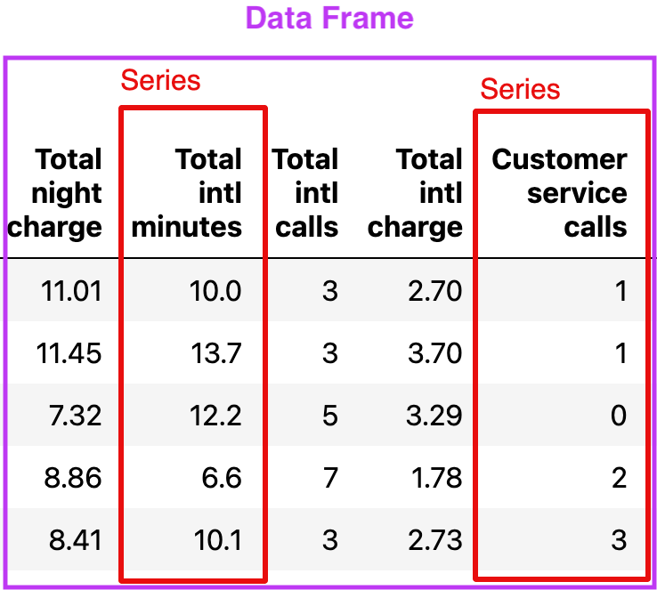
The core data structures in Pandas are Series and DataFrames. A Series is a one-dimensional indexed array of a single data type, while a DataFrame is a two-dimensional table where each column contains data of the same type. Think of a DataFrame as a collection of Series objects. DataFrames are ideal for representing real-world data, with each row representing an instance (such as an observation) and each column representing a feature of that instance.

import numpy as np
import pandas as pd

pd.set_option("display.precision", 2)

We demonstrate the main methods in action by analyzing a dataset on the churn rate of telecom operator clients. Let’s read the data (using the read_csv method), and take a look at the first 5 lines using the head method:

# for Jupyter-book, we copy data from GitHub. Locally, to save Internet traffic,
# you can specify the data/ folder from the root of your cloned
# https://github.com/Yorko/mlcourse.ai repo
DATA_URL = "https://raw.githubusercontent.com/Yorko/mlcourse.ai/main/data/"

df = pd.read_csv(DATA_URL + "telecom_churn.csv")
df.head()

	State	Account length	Area code	International plan	Voice mail plan	Number vmail messages	Total day minutes	Total day calls	Total day charge	Total eve minutes	Total eve calls	Total eve charge	Total night minutes	Total night calls	Total night charge	Total intl minutes	Total intl calls	Total intl charge	Customer service calls	Churn
0	KS	128	415	No	Yes	25	265.1	110	45.07	197.4	99	16.78	244.7	91	11.01	10.0	3	2.70	1	False
1	OH	107	415	No	Yes	26	161.6	123	27.47	195.5	103	16.62	254.4	103	11.45	13.7	3	3.70	1	False
2	NJ	137	415	No	No	0	243.4	114	41.38	121.2	110	10.30	162.6	104	7.32	12.2	5	3.29	0	False
3	OH	84	408	Yes	No	0	299.4	71	50.90	61.9	88	5.26	196.9	89	8.86	6.6	7	1.78	2	False
4	OK	75	415	Yes	No	0	166.7	113	28.34	148.3	122	12.61	186.9	121	8.41	10.1	3	2.73	3	False

Printing DataFrames in Jupyter notebooks

In Jupyter notebooks, Pandas DataFrames are printed as these pretty tables seen above while print(df.head()) is less nicely formatted. By default, Pandas displays 20 columns and 60 rows, so, if your DataFrame is bigger, use the set_option function as shown in the example below:

pd.set_option('display.max_columns', 100)
pd.set_option('display.max_rows', 100)

Recall that each row corresponds to one client, an instance, and columns are features of this instance.

Let’s have a look at data dimensionality, feature names, and feature types.

print(df.shape)

(3333, 20)

From the output, we can see that the table contains 3333 rows and 20 columns.

Now let’s try printing out column names using columns:

print(df.columns)

Index(['State', 'Account length', 'Area code', 'International plan',
       'Voice mail plan', 'Number vmail messages', 'Total day minutes',
       'Total day calls', 'Total day charge', 'Total eve minutes',
       'Total eve calls', 'Total eve charge', 'Total night minutes',
       'Total night calls', 'Total night charge', 'Total intl minutes',
       'Total intl calls', 'Total intl charge', 'Customer service calls',
       'Churn'],
      dtype='object')

We can use the info() method to output some general information about the dataframe:

print(df.info())

<class 'pandas.core.frame.DataFrame'>
RangeIndex: 3333 entries, 0 to 3332
Data columns (total 20 columns):
 #   Column                  Non-Null Count  Dtype  
---  ------                  --------------  -----  
 State                   3333 non-null   object 
 Account length          3333 non-null   int64  
 Area code               3333 non-null   int64  
 International plan      3333 non-null   object 
 Voice mail plan         3333 non-null   object 
 Number vmail messages   3333 non-null   int64  
 Total day minutes       3333 non-null   float64
 Total day calls         3333 non-null   int64  
 Total day charge        3333 non-null   float64
 Total eve minutes       3333 non-null   float64
Total eve calls         3333 non-null   int64  
Total eve charge        3333 non-null   float64
Total night minutes     3333 non-null   float64
Total night calls       3333 non-null   int64  
Total night charge      3333 non-null   float64
Total intl minutes      3333 non-null   float64
Total intl calls        3333 non-null   int64  
Total intl charge       3333 non-null   float64
Customer service calls  3333 non-null   int64  
Churn                   3333 non-null   bool   
dtypes: bool(1), float64(8), int64(8), object(3)
memory usage: 498.1+ KB
None

bool, int64, float64 and object are the data types of our features. We see that one feature is logical (bool), 3 features are of type object, and 16 features are numeric. With this same method, we can easily see if there are any missing values. Here, there are none because each column contains 3333 observations, the same number of rows we saw before with shape.

We can change the column type with the astype method. Let’s apply this method to the Churn feature to convert it into int64:

df["Churn"] = df["Churn"].astype("int64")

The describe method shows basic statistical characteristics of each numerical feature (int64 and float64 types): number of non-missing values, mean, standard deviation, range, median, 0.25 and 0.75 quartiles.

df.describe()

	Account length	Area code	Number vmail messages	Total day minutes	Total day calls	Total day charge	Total eve minutes	Total eve calls	Total eve charge	Total night minutes	Total night calls	Total night charge	Total intl minutes	Total intl calls	Total intl charge	Customer service calls	Churn
count	3333.00	3333.00	3333.00	3333.00	3333.00	3333.00	3333.00	3333.00	3333.00	3333.00	3333.00	3333.00	3333.00	3333.00	3333.00	3333.00	3333.00
mean	101.06	437.18	8.10	179.78	100.44	30.56	200.98	100.11	17.08	200.87	100.11	9.04	10.24	4.48	2.76	1.56	0.14
std	39.82	42.37	13.69	54.47	20.07	9.26	50.71	19.92	4.31	50.57	19.57	2.28	2.79	2.46	0.75	1.32	0.35
min	1.00	408.00	0.00	0.00	0.00	0.00	0.00	0.00	0.00	23.20	33.00	1.04	0.00	0.00	0.00	0.00	0.00
25%	74.00	408.00	0.00	143.70	87.00	24.43	166.60	87.00	14.16	167.00	87.00	7.52	8.50	3.00	2.30	1.00	0.00
50%	101.00	415.00	0.00	179.40	101.00	30.50	201.40	100.00	17.12	201.20	100.00	9.05	10.30	4.00	2.78	1.00	0.00
75%	127.00	510.00	20.00	216.40	114.00	36.79	235.30	114.00	20.00	235.30	113.00	10.59	12.10	6.00	3.27	2.00	0.00
max	243.00	510.00	51.00	350.80	165.00	59.64	363.70	170.00	30.91	395.00	175.00	17.77	20.00	20.00	5.40	9.00	1.00

In order to see statistics on non-numerical features, one has to explicitly indicate data types of interest in the include parameter.

df.describe(include=["object", "bool"])

	State	International plan	Voice mail plan
count	3333	3333	3333
unique	51	2	2
top	WV	No	No
freq	106	3010	2411

For categorical (type object) and boolean (type bool) features we can use the value_counts method. Let’s take a look at the distribution of Churn:

df["Churn"].value_counts()

0    2850
1     483
Name: Churn, dtype: int64

2850 users out of 3333 are loyal; their Churn value is 0. To calculate fractions, pass normalize=True to the value_counts function.

df["Churn"].value_counts(normalize=True)

0    0.86
1    0.14
Name: Churn, dtype: float64

Sorting#

A DataFrame can be sorted by the value of one of the variables (i.e columns). For example, we can sort by Total day charge (use ascending=False to sort in descending order):

df.sort_values(by="Total day charge", ascending=False).head()

	State	Account length	Area code	International plan	Voice mail plan	Total day minutes	Total day calls	Total day charge	Total eve minutes	Total eve calls	Total eve charge	Total night minutes	Total night calls	Total night charge	Total intl minutes	Total intl calls	Total intl charge	Customer service calls	Churn
365	CO	154	415	No	No	350.8	75	59.64	216.5	94	18.40	253.9	100	11.43	10.1	9	2.73	1	1
985	NY	64	415	Yes	No	346.8	55	58.96	249.5	79	21.21	275.4	102	12.39	13.3	9	3.59	1	1
2594	OH	115	510	Yes	No	345.3	81	58.70	203.4	106	17.29	217.5	107	9.79	11.8	8	3.19	1	1
156	OH	83	415	No	No	337.4	120	57.36	227.4	116	19.33	153.9	114	6.93	15.8	7	4.27	0	1
605	MO	112	415	No	No	335.5	77	57.04	212.5	109	18.06	265.0	132	11.93	12.7	8	3.43	2	1

We can also sort by multiple columns:

df.sort_values(by=["Churn", "Total day charge"], ascending=[True, False]).head()

	State	Account length	Area code	International plan	Voice mail plan	Number vmail messages	Total day minutes	Total day calls	Total day charge	Total eve minutes	Total eve calls	Total eve charge	Total night minutes	Total night calls	Total night charge	Total intl minutes	Total intl calls	Total intl charge	Customer service calls
688	MN	13	510	No	Yes	21	315.6	105	53.65	208.9	71	17.76	260.1	123	11.70	12.1	3	3.27	3
2259	NC	210	415	No	Yes	31	313.8	87	53.35	147.7	103	12.55	192.7	97	8.67	10.1	7	2.73	3
534	LA	67	510	No	No	0	310.4	97	52.77	66.5	123	5.65	246.5	99	11.09	9.2	10	2.48	4
575	SD	114	415	No	Yes	36	309.9	90	52.68	200.3	89	17.03	183.5	105	8.26	14.2	2	3.83	1
2858	AL	141	510	No	Yes	28	308.0	123	52.36	247.8	128	21.06	152.9	103	6.88	7.4	3	2.00	1

Indexing and retrieving data#

A DataFrame can be indexed in a few different ways.

To get a single column, you can use a DataFrame['Name'] construction. Let’s use this to answer a question about that column alone: what is the proportion of churned users in our dataframe?

df["Churn"].mean()

0.14491449144914492

14.5% is actually quite bad for a company; such a churn rate can make the company go bankrupt.

Boolean indexing with one column is also very convenient. The syntax is df[P(df['Name'])], where P is some logical condition that is checked for each element of the Name column. The result of such indexing is the DataFrame consisting only of the rows that satisfy the P condition on the Name column.

Let’s use it to answer the question:

What are the average values of numerical features for churned users?

Here we’l resort to an additional method select_dtypes to select all numeric columns.

df.select_dtypes(include=np.number)[df["Churn"] == 1].mean()

Account length            102.66
Area code                 437.82
Number vmail messages       5.12
Total day minutes         206.91
Total day calls           101.34
Total day charge           35.18
Total eve minutes         212.41
Total eve calls           100.56
Total eve charge           18.05
Total night minutes       205.23
Total night calls         100.40
Total night charge          9.24
Total intl minutes         10.70
Total intl calls            4.16
Total intl charge           2.89
Customer service calls      2.23
Churn                       1.00
dtype: float64

How much time (on average) do churned users spend on the phone during daytime?

df[df["Churn"] == 1]["Total day minutes"].mean()

206.91407867494823

What is the maximum length of international calls among loyal users (Churn == 0) who do not have an international plan?

df[(df["Churn"] == 0) & (df["International plan"] == "No")]["Total intl minutes"].max()

18.9

DataFrames can be indexed by column name (label) or row name (index) or by the serial number of a row. The loc method is used for indexing by name, while iloc() is used for indexing by number.

In the first case below, we say “give us the values of the rows with index from 0 to 5 (inclusive) and columns labeled from State to Area code (inclusive)”. In the second case, we say “give us the values of the first five rows in the first three columns” (as in a typical Python slice: the maximal value is not included).

df.loc[0:5, "State":"Area code"]

	State	Account length	Area code
0	KS	128	415
1	OH	107	415
2	NJ	137	415
3	OH	84	408
4	OK	75	415
5	AL	118	510

df.iloc[0:5, 0:3]

	State	Account length	Area code
0	KS	128	415
1	OH	107	415
2	NJ	137	415
3	OH	84	408
4	OK	75	415

If we need the first or the last line of the data frame, we can use the df[:1] or df[-1:] construction:

df[-1:]

	State	Account length	Area code	International plan	Voice mail plan	Number vmail messages	Total day minutes	Total day calls	Total day charge	Total eve minutes	Total eve calls	Total eve charge	Total night minutes	Total night calls	Total night charge	Total intl minutes	Total intl calls	Total intl charge	Customer service calls	Churn
3332	TN	74	415	No	Yes	25	234.4	113	39.85	265.9	82	22.6	241.4	77	10.86	13.7	4	3.7	0	0

Applying Functions to Cells, Columns and Rows#

To apply functions to each column, use apply():

df.apply(np.max)

State                        WY
Account length              243
Area code                   510
International plan          Yes
Voice mail plan             Yes
Number vmail messages        51
Total day minutes         350.8
Total day calls             165
Total day charge          59.64
Total eve minutes         363.7
Total eve calls             170
Total eve charge          30.91
Total night minutes       395.0
Total night calls           175
Total night charge        17.77
Total intl minutes         20.0
Total intl calls             20
Total intl charge           5.4
Customer service calls        9
Churn                         1
dtype: object

The apply method can also be used to apply a function to each row. To do this, specify axis=1. Lambda functions are very convenient in such scenarios. For example, if we need to select all states starting with ‘W’, we can do it like this:

df[df["State"].apply(lambda state: state[0] == "W")].head()

	State	Account length	Area code	International plan	Voice mail plan	Number vmail messages	Total day minutes	Total day calls	Total day charge	Total eve minutes	Total eve calls	Total eve charge	Total night minutes	Total night calls	Total night charge	Total intl minutes	Total intl calls	Total intl charge	Customer service calls	Churn
9	WV	141	415	Yes	Yes	37	258.6	84	43.96	222.0	111	18.87	326.4	97	14.69	11.2	5	3.02	0	0
26	WY	57	408	No	Yes	39	213.0	115	36.21	191.1	112	16.24	182.7	115	8.22	9.5	3	2.57	0	0
44	WI	64	510	No	No	0	154.0	67	26.18	225.8	118	19.19	265.3	86	11.94	3.5	3	0.95	1	0
49	WY	97	415	No	Yes	24	133.2	135	22.64	217.2	58	18.46	70.6	79	3.18	11.0	3	2.97	1	0
54	WY	87	415	No	No	0	151.0	83	25.67	219.7	116	18.67	203.9	127	9.18	9.7	3	2.62	5	1

The map method can be used to replace values in a column by passing a dictionary of the form {old_value: new_value} as its argument:

d = {"No": False, "Yes": True}
df["International plan"] = df["International plan"].map(d)
df.head()

	State	Account length	Area code	International plan	Voice mail plan	Number vmail messages	Total day minutes	Total day calls	Total day charge	Total eve minutes	Total eve calls	Total eve charge	Total night minutes	Total night calls	Total night charge	Total intl minutes	Total intl calls	Total intl charge	Customer service calls
0	KS	128	415	False	Yes	25	265.1	110	45.07	197.4	99	16.78	244.7	91	11.01	10.0	3	2.70	1
1	OH	107	415	False	Yes	26	161.6	123	27.47	195.5	103	16.62	254.4	103	11.45	13.7	3	3.70	1
2	NJ	137	415	False	No	0	243.4	114	41.38	121.2	110	10.30	162.6	104	7.32	12.2	5	3.29	0
3	OH	84	408	True	No	0	299.4	71	50.90	61.9	88	5.26	196.9	89	8.86	6.6	7	1.78	2
4	OK	75	415	True	No	0	166.7	113	28.34	148.3	122	12.61	186.9	121	8.41	10.1	3	2.73	3

Almost the same thing can be done with the replace method.

Difference in treating values that are absent in the mapping dictionary

There's a slight difference. Еру `replace` method will not do anything with values not found in the mapping dictionary, while `map` will change them to NaNs).

a_series = pd.Series(['a', 'b', 'c'])
a_series.replace({'a': 1, 'b': 1})     # 1, 2, c
a_series.map({'a': 1, 'b': 2})     # 1, 2, NaN

  1.0
  2.0
  NaN
dtype: float64

df = df.replace({"Voice mail plan": d})
df.head()

	State	Account length	Area code	International plan	Voice mail plan	Number vmail messages	Total day minutes	Total day calls	Total day charge	Total eve minutes	Total eve calls	Total eve charge	Total night minutes	Total night calls	Total night charge	Total intl minutes	Total intl calls	Total intl charge	Customer service calls
0	KS	128	415	False	True	25	265.1	110	45.07	197.4	99	16.78	244.7	91	11.01	10.0	3	2.70	1
1	OH	107	415	False	True	26	161.6	123	27.47	195.5	103	16.62	254.4	103	11.45	13.7	3	3.70	1
2	NJ	137	415	False	False	0	243.4	114	41.38	121.2	110	10.30	162.6	104	7.32	12.2	5	3.29	0
3	OH	84	408	True	False	0	299.4	71	50.90	61.9	88	5.26	196.9	89	8.86	6.6	7	1.78	2
4	OK	75	415	True	False	0	166.7	113	28.34	148.3	122	12.61	186.9	121	8.41	10.1	3	2.73	3

Grouping#

In general, grouping data in Pandas works as follows:

df.groupby(by=grouping_columns)[columns_to_show].function()

First, the groupby method divides the grouping_columns by their values. They become a new index in the resulting dataframe.
Then, columns of interest are selected (columns_to_show). If columns_to_show is not included, all non groupby clauses will be included.
Finally, one or several functions are applied to the obtained groups per selected columns.

Here is an example where we group the data according to the values of the Churn variable and display statistics of three columns in each group:

columns_to_show = ["Total day minutes", "Total eve minutes", "Total night minutes"]

df.groupby(["Churn"])[columns_to_show].describe(percentiles=[])

	Total day minutes						Total eve minutes						Total night minutes
	count	mean	std	min	50%	max	count	mean	std	min	50%	max	count	mean	std	min	50%	max
Churn
0	2850.0	175.18	50.18	0.0	177.2	315.6	2850.0	199.04	50.29	0.0	199.6	361.8	2850.0	200.13	51.11	23.2	200.25	395.0
1	483.0	206.91	69.00	0.0	217.6	350.8	483.0	212.41	51.73	70.9	211.3	363.7	483.0	205.23	47.13	47.4	204.80	354.9

Let’s do the same thing, but slightly differently by passing a list of functions to agg():

columns_to_show = ["Total day minutes", "Total eve minutes", "Total night minutes"]

df.groupby(["Churn"])[columns_to_show].agg([np.mean, np.std, np.min, np.max])

	Total day minutes				Total eve minutes				Total night minutes
	mean	std	amin	amax	mean	std	amin	amax	mean	std	amin	amax
Churn
0	175.18	50.18	0.0	315.6	199.04	50.29	0.0	361.8	200.13	51.11	23.2	395.0
1	206.91	69.00	0.0	350.8	212.41	51.73	70.9	363.7	205.23	47.13	47.4	354.9

Summary tables#

Suppose we want to see how the observations in our dataset are distributed in the context of two variables – Churn and International plan. To do so, we can build a contingency table using the crosstab method:

pd.crosstab(df["Churn"], df["International plan"])

International plan	False	True
Churn
0	2664	186
1	346	137

pd.crosstab(df["Churn"], df["Voice mail plan"], normalize=True)

Voice mail plan	False	True
Churn
0	0.60	0.25
1	0.12	0.02

We can see that most of the users are loyal and do not use additional services (International Plan/Voice mail).

This will resemble pivot tables to those familiar with Excel. And, of course, pivot tables are implemented in Pandas: the pivot_table method takes the following parameters:

values – a list of variables to calculate statistics for,
index – a list of variables to group data by,
aggfunc – what statistics we need to calculate for groups, e.g. sum, mean, maximum, minimum or something else.

Let’s take a look at the average number of day, evening, and night calls by area code:

df.pivot_table(
    ["Total day calls", "Total eve calls", "Total night calls"],
    ["Area code"],
    aggfunc="mean",
)

	Total day calls	Total eve calls	Total night calls
Area code
408	100.50	99.79	99.04
415	100.58	100.50	100.40
510	100.10	99.67	100.60

DataFrame transformations#

Like many other things in Pandas, adding columns to a DataFrame is doable in many ways.

For example, if we want to calculate the total number of calls for all users, let’s create the total_calls Series and paste it into the DataFrame:

total_calls = (
    df["Total day calls"]
    + df["Total eve calls"]
    + df["Total night calls"]
    + df["Total intl calls"]
)
df.insert(loc=len(df.columns), column="Total calls", value=total_calls)
# loc parameter is the number of columns after which to insert the Series object
# we set it to len(df.columns) to paste it at the very end of the dataframe
df.head()

	State	Account length	Area code	International plan	Voice mail plan	Number vmail messages	Total day minutes	Total day calls	Total day charge	Total eve minutes	Total eve calls	Total eve charge	Total night minutes	Total night calls	Total night charge	Total intl minutes	Total intl calls	Total intl charge	Customer service calls	Total calls
0	KS	128	415	False	True	25	265.1	110	45.07	197.4	99	16.78	244.7	91	11.01	10.0	3	2.70	1	303
1	OH	107	415	False	True	26	161.6	123	27.47	195.5	103	16.62	254.4	103	11.45	13.7	3	3.70	1	332
2	NJ	137	415	False	False	0	243.4	114	41.38	121.2	110	10.30	162.6	104	7.32	12.2	5	3.29	0	333
3	OH	84	408	True	False	0	299.4	71	50.90	61.9	88	5.26	196.9	89	8.86	6.6	7	1.78	2	255
4	OK	75	415	True	False	0	166.7	113	28.34	148.3	122	12.61	186.9	121	8.41	10.1	3	2.73	3	359

It is possible to add a column more easily without creating an intermediate Series instance:

df["Total charge"] = (
    df["Total day charge"]
    + df["Total eve charge"]
    + df["Total night charge"]
    + df["Total intl charge"]
)
df.head()

	State	Account length	Area code	International plan	Voice mail plan	Number vmail messages	Total day minutes	Total day calls	Total day charge	Total eve minutes	Total eve calls	Total eve charge	Total night minutes	Total night calls	Total night charge	Total intl minutes	Total intl calls	Total intl charge	Customer service calls	Total calls	Total charge
0	KS	128	415	False	True	25	265.1	110	45.07	197.4	99	16.78	244.7	91	11.01	10.0	3	2.70	1	303	75.56
1	OH	107	415	False	True	26	161.6	123	27.47	195.5	103	16.62	254.4	103	11.45	13.7	3	3.70	1	332	59.24
2	NJ	137	415	False	False	0	243.4	114	41.38	121.2	110	10.30	162.6	104	7.32	12.2	5	3.29	0	333	62.29
3	OH	84	408	True	False	0	299.4	71	50.90	61.9	88	5.26	196.9	89	8.86	6.6	7	1.78	2	255	66.80
4	OK	75	415	True	False	0	166.7	113	28.34	148.3	122	12.61	186.9	121	8.41	10.1	3	2.73	3	359	52.09

To delete columns or rows, use the drop method, passing the required indexes and the axis parameter (1 if you delete columns, and nothing or 0 if you delete rows). The inplace argument tells whether to change the original DataFrame. With inplace=False, the drop method doesn’t change the existing DataFrame and returns a new one with dropped rows or columns. With inplace=True, it alters the DataFrame.

# get rid of just created columns
df.drop(["Total charge", "Total calls"], axis=1, inplace=True)
# and here’s how you can delete rows
df.drop([1, 2]).head()

	State	Account length	Area code	International plan	Voice mail plan	Number vmail messages	Total day minutes	Total day calls	Total day charge	Total eve minutes	Total eve calls	Total eve charge	Total night minutes	Total night calls	Total night charge	Total intl minutes	Total intl calls	Total intl charge	Customer service calls
0	KS	128	415	False	True	25	265.1	110	45.07	197.4	99	16.78	244.7	91	11.01	10.0	3	2.70	1
3	OH	84	408	True	False	0	299.4	71	50.90	61.9	88	5.26	196.9	89	8.86	6.6	7	1.78	2
4	OK	75	415	True	False	0	166.7	113	28.34	148.3	122	12.61	186.9	121	8.41	10.1	3	2.73	3
5	AL	118	510	True	False	0	223.4	98	37.98	220.6	101	18.75	203.9	118	9.18	6.3	6	1.70	0
6	MA	121	510	False	True	24	218.2	88	37.09	348.5	108	29.62	212.6	118	9.57	7.5	7	2.03	3

2. First attempt at predicting telecom churn#

Let’s see how churn rate is related to the International plan feature. We’ll do this using a crosstab contingency table and also through visual analysis with Seaborn (however, visual analysis will be covered more thoroughly in the next topic).

pd.crosstab(df["Churn"], df["International plan"], margins=True)

International plan	False	True	All
Churn
0	2664	186	2850
1	346	137	483
All	3010	323	3333

# some imports to set up plotting
import matplotlib.pyplot as plt

# !pip install seaborn
import seaborn as sns

# import some nice vis settings
sns.set()
# Graphics in the Retina format are more sharp and legible
%config InlineBackend.figure_format = 'retina'

sns.countplot(x="International plan", hue="Churn", data=df);

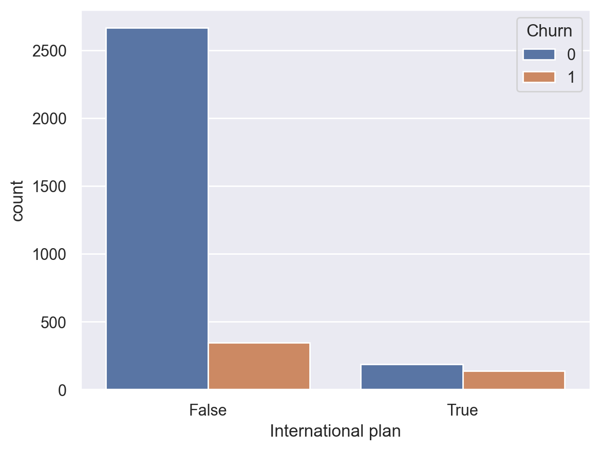
../../_images/f75fdb20aa8b3c2c266e5cd91185404a30fe9c6c995742c0589f9dc9372fe2cb.png

We observe that the churn rate is significantly higher with the International Plan. This is a noteworthy finding. Perhaps, high and poorly managed expenses for international calls cause conflicts and result in discontent among the telecom operator’s customers.

Next, let’s look at another important feature – Customer service calls. Let’s also make a summary table and a picture.

pd.crosstab(df["Churn"], df["Customer service calls"], margins=True)

Customer service calls	0	1	2	3	4	5	6	7	8	9	All
Churn
0	605	1059	672	385	90	26	8	4	1	0	2850
1	92	122	87	44	76	40	14	5	1	2	483
All	697	1181	759	429	166	66	22	9	2	2	3333

sns.countplot(x="Customer service calls", hue="Churn", data=df);

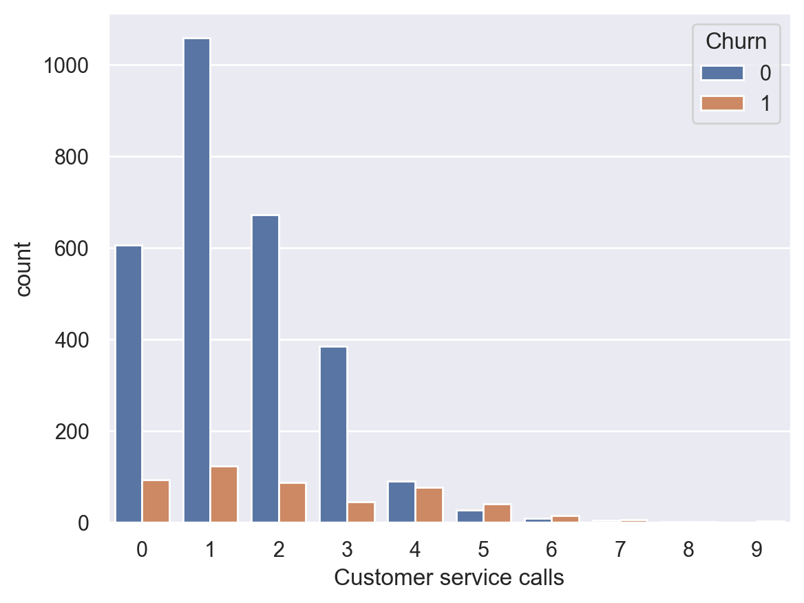
../../_images/80e372b115236adc458830788295c82440046d52cb2fe260cb7eaa106e78abf5.png

Although it’s not so obvious from the summary table, it’s easy to see from the above plot that the churn rate increases sharply from 4 customer service calls and above.

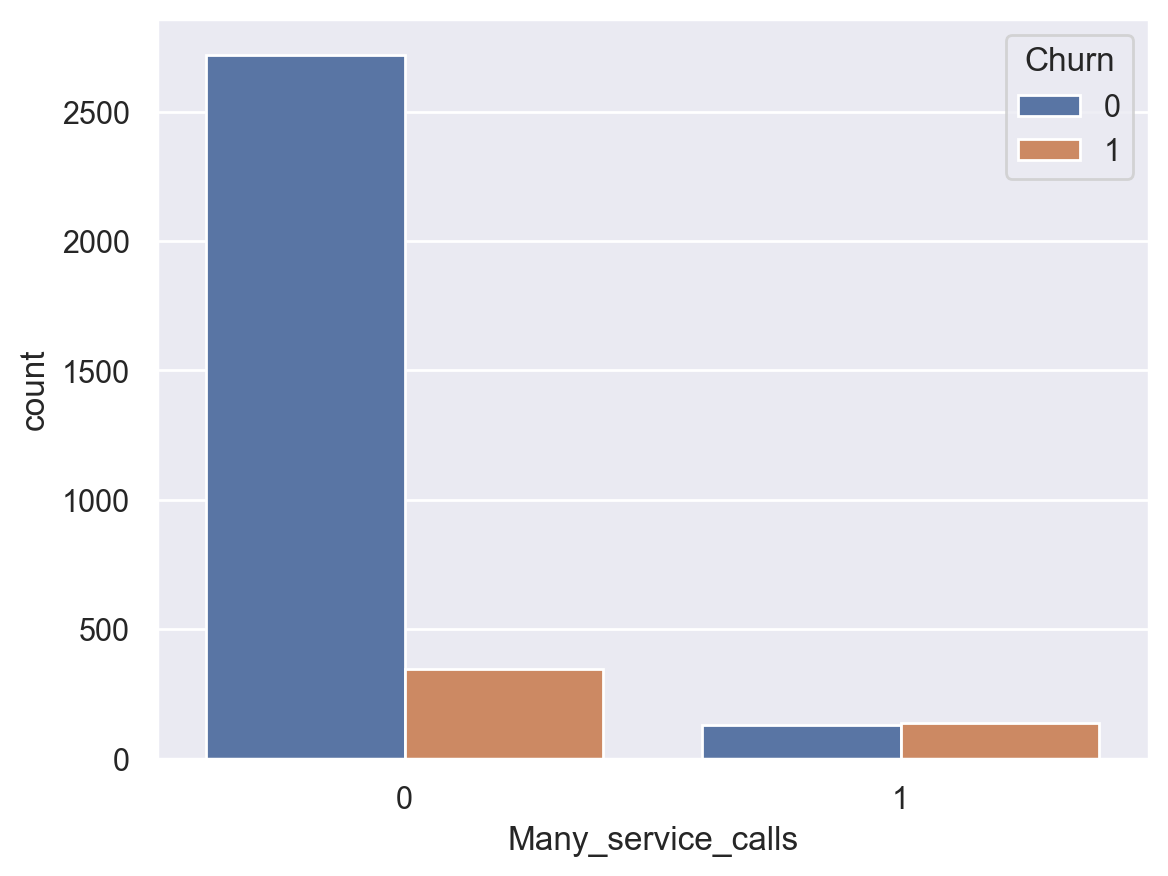
Now let’s add a binary feature to our DataFrame – Customer service calls > 3. And once again, let’s see how it relates to churn.

df["Many_service_calls"] = (df["Customer service calls"] > 3).astype("int")

pd.crosstab(df["Many_service_calls"], df["Churn"], margins=True)

Churn	0	1	All
Many_service_calls
0	2721	345	3066
1	129	138	267
All	2850	483	3333

sns.countplot(x="Many_service_calls", hue="Churn", data=df);

../../_images/7bf4cada9d6b2686bbe573a1760e9b37037a86566f1b40c2516e0f819580bb25.png

Let’s construct another contingency table that relates Churn with both the International plan and the freshly created Many_service_calls feature.

pd.crosstab(df["Many_service_calls"] & df["International plan"], df["Churn"], margins=True)

Churn	0	1	All
row_0
False	2841	464	3305
True	9	19	28
All	2850	483	3333

Thus, by predicting that a customer will not remain loyal (Churn=1) if they have made more than 3 calls to the service center AND have added the International Plan, and predicting Churn=0 otherwise (and “otherwise” here means negation, i.e. Many_service_calls <= 3 OR International Plan is not added ), we anticipate an accuracy of 85.8% (we will only be incorrect 464 + 9 times, look at the contingency table above; and \(1 - \frac{464 + 9}{3333} \approx 85.8\%\)). This 85.8% accuracy, obtained through such straightforward reasoning, serves as a useful starting point (baseline) for the development of future machine learning models.

As we move on through this course, recall that, before the advent of machine learning, the data analysis process looked something like this. Let’s recap what we’ve covered:

The share of loyal clients in the dataset is 85.5%. The most naive model that always predicts a “loyal customer” on such data will guess right in about 85.5% of all cases. That is, the proportion of correct answers (accuracy) of subsequent models should be no less than this number, and will hopefully be significantly higher;
With the help of a simple prediction that can be expressed by the following formula: International plan = True & Customer Service calls > 3 => Churn = 1, else Churn = 0, we can expect a guessing rate of 85.8%, which is just above 85.5%. Subsequently, we’ll talk about decision trees and figure out how to find such rules automatically based only on the input data;
We got these two baselines without applying machine learning, and they’ll serve as the starting point for our subsequent models. If it turns out that with enormous effort, we increase accuracy by only 0.5%, persay, then possibly we are doing something wrong, and it suffices to confine ourselves to a simple “if-else” model with two conditions;
Before training complex models, it is recommended to wrangle the data a bit, make some plots, and check simple assumptions. Moreover, in business applications of machine learning, they usually start with simple solutions and then experiment with more complex ones.

3. Useful resources#

The same notebook as an interactive web-based Kaggle Kernel
“Merging DataFrames with pandas” – a tutorial by Max Plako within mlcourse.ai (the full list of tutorials is here)
“Handle different dataset with dask and trying a little dask ML” – a tutorial by Irina Knyazeva within mlcourse.ai
Course repo, and YouTube channel
Official Pandas documentation
Course materials as a Kaggle Dataset

If you read Russian: an article on Habr with ~ the same material. And a lecture on YouTube
10 minutes to pandas
Pandas cheatsheet PDF
GitHub repos: Pandas exercises and “Effective Pandas”
scipy-lectures.org – tutorials on pandas, numpy, matplotlib and scikit-learn