Assignment #3 (demo). Decision trees with a toy task and the UCI Adult dataset#

Authors: Maria Kuna (Sumarokova), and Yury Kashnitsky. Translated and edited by Gleb Filatov, Aleksey Kiselev, Anastasia Manokhina, Egor Polusmak, and Yuanyuan Pao. All content is distributed under the Creative Commons CC BY-NC-SA 4.0 license.
Same assignment as a Kaggle Kernel + solution. Fill in the answers in the web-form.
Let’s start by loading all necessary libraries:
import collections
from io import StringIO

import numpy as np
import pandas as pd
import pydotplus  # pip install pydotplus
import seaborn as sns
from ipywidgets import Image
from sklearn import preprocessing
from sklearn.ensemble import RandomForestClassifier
from sklearn.metrics import accuracy_score
from sklearn.model_selection import GridSearchCV
from sklearn.preprocessing import LabelEncoder
from sklearn.tree import DecisionTreeClassifier, export_graphviz

from matplotlib import pyplot as plt
plt.rcParams["figure.figsize"] = (10, 8)
Part 1. Toy dataset “Will They? Won’t They?”#
Your goal is to figure out how decision trees work by walking through a toy problem. While a single decision tree does not yield outstanding results, other performant algorithms like gradient boosting and random forests are based on the same idea. That is why knowing how decision trees work might be useful.
We’ll go through a toy example of binary classification - Person A is deciding whether they will go on a second date with Person B. It will depend on their looks, eloquence, alcohol consumption (only for example), and how much money was spent on the first date.
Creating the dataset#
# Create dataframe with dummy variables
def create_df(dic, feature_list):
    out = pd.DataFrame(dic)
    out = pd.concat([out, pd.get_dummies(out[feature_list])], axis=1)
    out.drop(feature_list, axis=1, inplace=True)
    return out


# Some feature values are present in train and absent in test and vice-versa.
def intersect_features(train, test):
    common_feat = list(set(train.keys()) & set(test.keys()))
    return train[common_feat], test[common_feat]
features = ["Looks", "Alcoholic_beverage", "Eloquence", "Money_spent"]
Training data#
df_train = {}
df_train["Looks"] = [
    "handsome",
    "handsome",
    "handsome",
    "repulsive",
    "repulsive",
    "repulsive",
    "handsome",
]
df_train["Alcoholic_beverage"] = ["yes", "yes", "no", "no", "yes", "yes", "yes"]
df_train["Eloquence"] = ["high", "low", "average", "average", "low", "high", "average"]
df_train["Money_spent"] = ["lots", "little", "lots", "little", "lots", "lots", "lots"]
df_train["Will_go"] = LabelEncoder().fit_transform(["+", "-", "+", "-", "-", "+", "+"])

df_train = create_df(df_train, features)
df_train
| Will_go | Looks_handsome | Looks_repulsive | Alcoholic_beverage_no | Alcoholic_beverage_yes | Eloquence_average | Eloquence_high | Eloquence_low | Money_spent_little | Money_spent_lots | |
|---|---|---|---|---|---|---|---|---|---|---|
| 0 | 0 | True | False | False | True | False | True | False | False | True |
| 1 | 1 | True | False | False | True | False | False | True | True | False |
| 2 | 0 | True | False | True | False | True | False | False | False | True |
| 3 | 1 | False | True | True | False | True | False | False | True | False |
| 4 | 1 | False | True | False | True | False | False | True | False | True |
| 5 | 0 | False | True | False | True | False | True | False | False | True |
| 6 | 0 | True | False | False | True | True | False | False | False | True |
Test data#
df_test = {}
df_test["Looks"] = ["handsome", "handsome", "repulsive"]
df_test["Alcoholic_beverage"] = ["no", "yes", "yes"]
df_test["Eloquence"] = ["average", "high", "average"]
df_test["Money_spent"] = ["lots", "little", "lots"]
df_test = create_df(df_test, features)
df_test
| Looks_handsome | Looks_repulsive | Alcoholic_beverage_no | Alcoholic_beverage_yes | Eloquence_average | Eloquence_high | Money_spent_little | Money_spent_lots | |
|---|---|---|---|---|---|---|---|---|
| 0 | True | False | True | False | True | False | False | True |
| 1 | True | False | False | True | False | True | True | False |
| 2 | False | True | False | True | True | False | False | True |
# Some feature values are present in train and absent in test and vice-versa.
y = df_train["Will_go"]
df_train, df_test = intersect_features(train=df_train, test=df_test)
df_train
| Alcoholic_beverage_yes | Looks_repulsive | Looks_handsome | Alcoholic_beverage_no | Eloquence_average | Eloquence_high | Money_spent_lots | Money_spent_little | |
|---|---|---|---|---|---|---|---|---|
| 0 | True | False | True | False | False | True | True | False |
| 1 | True | False | True | False | False | False | False | True |
| 2 | False | False | True | True | True | False | True | False |
| 3 | False | True | False | True | True | False | False | True |
| 4 | True | True | False | False | False | False | True | False |
| 5 | True | True | False | False | False | True | True | False |
| 6 | True | False | True | False | True | False | True | False |
df_test
| Alcoholic_beverage_yes | Looks_repulsive | Looks_handsome | Alcoholic_beverage_no | Eloquence_average | Eloquence_high | Money_spent_lots | Money_spent_little | |
|---|---|---|---|---|---|---|---|---|
| 0 | False | False | True | True | True | False | True | False |
| 1 | True | False | True | False | False | True | False | True |
| 2 | True | True | False | False | True | False | True | False |
Draw a decision tree (by hand or in any graphics editor) for this dataset. Optionally you can also implement tree construction and draw it here.#
1. What is the entropy \(S_0\) of the initial system? By system states, we mean values of the binary feature “Will_go” - 0 or 1 - two states in total.
# You code here (read-only in a JupyterBook, pls run jupyter-notebook to edit)
2. Let’s split the data by the feature “Looks_handsome”. What is the entropy \(S_1\) of the left group - the one with “Looks_handsome”. What is the entropy \(S_2\) in the opposite group? What is the information gain (IG) if we consider such a split?
# You code here (read-only in a JupyterBook, pls run jupyter-notebook to edit)
Train a decision tree using sklearn on the training data. You may choose any depth for the tree.#
# You code here (read-only in a JupyterBook, pls run jupyter-notebook to edit)
Additional: display the resulting tree using graphviz. You can use pydot or a web-service, e.g. this one.#
# You code here (read-only in a JupyterBook, pls run jupyter-notebook to edit)
Part 2. Functions for calculating entropy and information gain.#
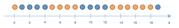
Consider the following warm-up example: we have 9 blue balls and 11 yellow balls. Let ball have label 1 if it is blue, 0 otherwise.
balls = [1 for i in range(9)] + [0 for i in range(11)]
Next split the balls into two groups:
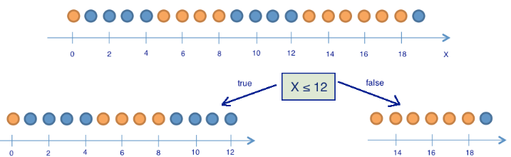
# two groups
balls_left = [1 for i in range(8)] + [0 for i in range(5)]  # 8 blue and 5 yellow
balls_right = [1 for i in range(1)] + [0 for i in range(6)]  # 1 blue and 6 yellow
Implement a function to calculate the Shannon Entropy#
def entropy(a_list):
    # You code here (read-only in a JupyterBook, pls run jupyter-notebook to edit)
    pass
Tests
print(entropy(balls))  # 9 blue и 11 yellow
print(entropy(balls_left))  # 8 blue и 5 yellow
print(entropy(balls_right))  # 1 blue и 6 yellow
print(entropy([1, 2, 3, 4, 5, 6]))  # entropy of a fair 6-sided die
None
None
None
None
3. What is the entropy of the state given by the list balls_left?
4. What is the entropy of a fair die? (where we look at a die as a system with 6 equally probable states)?
# information gain calculation
def information_gain(root, left, right):
    """ root - initial data, left and right - two partitions of initial data"""

    # You code here (read-only in a JupyterBook, pls run jupyter-notebook to edit)
    pass
5. What is the information gain from splitting the initial dataset into balls_left and balls_right ?
def information_gains(X, y):
    """Outputs information gain when splitting with each feature"""

    # You code here (read-only in a JupyterBook, pls run jupyter-notebook to edit)
    pass
Optional:#
Implement a decision tree building algorithm by calling
information_gainsrecursivelyPlot the resulting tree
Part 3. The “Adult” dataset#
Dataset description:
Dataset UCI Adult (no need to download it, we have a copy in the course repository): classify people using demographic data - whether they earn more than $50,000 per year or not.
Feature descriptions:
Age – continuous feature
Workclass – continuous feature
fnlwgt – final weight of object, continuous feature
Education – categorical feature
Education_Num – number of years of education, continuous feature
Martial_Status – categorical feature
Occupation – categorical feature
Relationship – categorical feature
Race – categorical feature
Sex – categorical feature
Capital_Gain – continuous feature
Capital_Loss – continuous feature
Hours_per_week – continuous feature
Country – categorical feature
Target – earnings level, categorical (binary) feature.
Reading train and test data
# for Jupyter-book, we copy data from GitHub, locally, to save Internet traffic,
# you can specify the data/ folder from the root of your cloned
# https://github.com/Yorko/mlcourse.ai repo, to save Internet traffic
DATA_PATH = "https://raw.githubusercontent.com/Yorko/mlcourse.ai/main/data/"
data_train = pd.read_csv(DATA_PATH + "adult_train.csv", sep=";")
data_train.tail()
| Age | Workclass | fnlwgt | Education | Education_Num | Martial_Status | Occupation | Relationship | Race | Sex | Capital_Gain | Capital_Loss | Hours_per_week | Country | Target | |
|---|---|---|---|---|---|---|---|---|---|---|---|---|---|---|---|
| 32556 | 27 | Private | 257302 | Assoc-acdm | 12 | Married-civ-spouse | Tech-support | Wife | White | Female | 0 | 0 | 38 | United-States | <=50K |
| 32557 | 40 | Private | 154374 | HS-grad | 9 | Married-civ-spouse | Machine-op-inspct | Husband | White | Male | 0 | 0 | 40 | United-States | >50K |
| 32558 | 58 | Private | 151910 | HS-grad | 9 | Widowed | Adm-clerical | Unmarried | White | Female | 0 | 0 | 40 | United-States | <=50K |
| 32559 | 22 | Private | 201490 | HS-grad | 9 | Never-married | Adm-clerical | Own-child | White | Male | 0 | 0 | 20 | United-States | <=50K |
| 32560 | 52 | Self-emp-inc | 287927 | HS-grad | 9 | Married-civ-spouse | Exec-managerial | Wife | White | Female | 15024 | 0 | 40 | United-States | >50K |
data_test = pd.read_csv(DATA_PATH + "adult_test.csv", sep=";")
data_test.tail()
| Age | Workclass | fnlwgt | Education | Education_Num | Martial_Status | Occupation | Relationship | Race | Sex | Capital_Gain | Capital_Loss | Hours_per_week | Country | Target | |
|---|---|---|---|---|---|---|---|---|---|---|---|---|---|---|---|
| 16277 | 39 | Private | 215419.0 | Bachelors | 13.0 | Divorced | Prof-specialty | Not-in-family | White | Female | 0.0 | 0.0 | 36.0 | United-States | <=50K. |
| 16278 | 64 | NaN | 321403.0 | HS-grad | 9.0 | Widowed | NaN | Other-relative | Black | Male | 0.0 | 0.0 | 40.0 | United-States | <=50K. |
| 16279 | 38 | Private | 374983.0 | Bachelors | 13.0 | Married-civ-spouse | Prof-specialty | Husband | White | Male | 0.0 | 0.0 | 50.0 | United-States | <=50K. |
| 16280 | 44 | Private | 83891.0 | Bachelors | 13.0 | Divorced | Adm-clerical | Own-child | Asian-Pac-Islander | Male | 5455.0 | 0.0 | 40.0 | United-States | <=50K. |
| 16281 | 35 | Self-emp-inc | 182148.0 | Bachelors | 13.0 | Married-civ-spouse | Exec-managerial | Husband | White | Male | 0.0 | 0.0 | 60.0 | United-States | >50K. |
# necessary to remove rows with incorrect labels in test dataset
data_test = data_test[
    (data_test["Target"] == " >50K.") | (data_test["Target"] == " <=50K.")
]

# encode target variable as integer
data_train.loc[data_train["Target"] == " <=50K", "Target"] = 0
data_train.loc[data_train["Target"] == " >50K", "Target"] = 1

data_test.loc[data_test["Target"] == " <=50K.", "Target"] = 0
data_test.loc[data_test["Target"] == " >50K.", "Target"] = 1
Primary data analysis
data_test.describe(include="all").T
| count | unique | top | freq | mean | std | min | 25% | 50% | 75% | max | |
|---|---|---|---|---|---|---|---|---|---|---|---|
| Age | 16281 | 73 | 35 | 461 | NaN | NaN | NaN | NaN | NaN | NaN | NaN |
| Workclass | 15318 | 8 | Private | 11210 | NaN | NaN | NaN | NaN | NaN | NaN | NaN |
| fnlwgt | 16281.0 | NaN | NaN | NaN | 189435.677784 | 105714.907671 | 13492.0 | 116736.0 | 177831.0 | 238384.0 | 1490400.0 |
| Education | 16281 | 16 | HS-grad | 5283 | NaN | NaN | NaN | NaN | NaN | NaN | NaN |
| Education_Num | 16281.0 | NaN | NaN | NaN | 10.072907 | 2.567545 | 1.0 | 9.0 | 10.0 | 12.0 | 16.0 |
| Martial_Status | 16281 | 7 | Married-civ-spouse | 7403 | NaN | NaN | NaN | NaN | NaN | NaN | NaN |
| Occupation | 15315 | 14 | Prof-specialty | 2032 | NaN | NaN | NaN | NaN | NaN | NaN | NaN |
| Relationship | 16281 | 6 | Husband | 6523 | NaN | NaN | NaN | NaN | NaN | NaN | NaN |
| Race | 16281 | 5 | White | 13946 | NaN | NaN | NaN | NaN | NaN | NaN | NaN |
| Sex | 16281 | 2 | Male | 10860 | NaN | NaN | NaN | NaN | NaN | NaN | NaN |
| Capital_Gain | 16281.0 | NaN | NaN | NaN | 1081.905104 | 7583.935968 | 0.0 | 0.0 | 0.0 | 0.0 | 99999.0 |
| Capital_Loss | 16281.0 | NaN | NaN | NaN | 87.899269 | 403.105286 | 0.0 | 0.0 | 0.0 | 0.0 | 3770.0 |
| Hours_per_week | 16281.0 | NaN | NaN | NaN | 40.392236 | 12.479332 | 1.0 | 40.0 | 40.0 | 45.0 | 99.0 |
| Country | 16007 | 40 | United-States | 14662 | NaN | NaN | NaN | NaN | NaN | NaN | NaN |
| Target | 16281.0 | 2.0 | 0.0 | 12435.0 | NaN | NaN | NaN | NaN | NaN | NaN | NaN |
data_train["Target"].value_counts()
Target
0    24720
1     7841
Name: count, dtype: int64
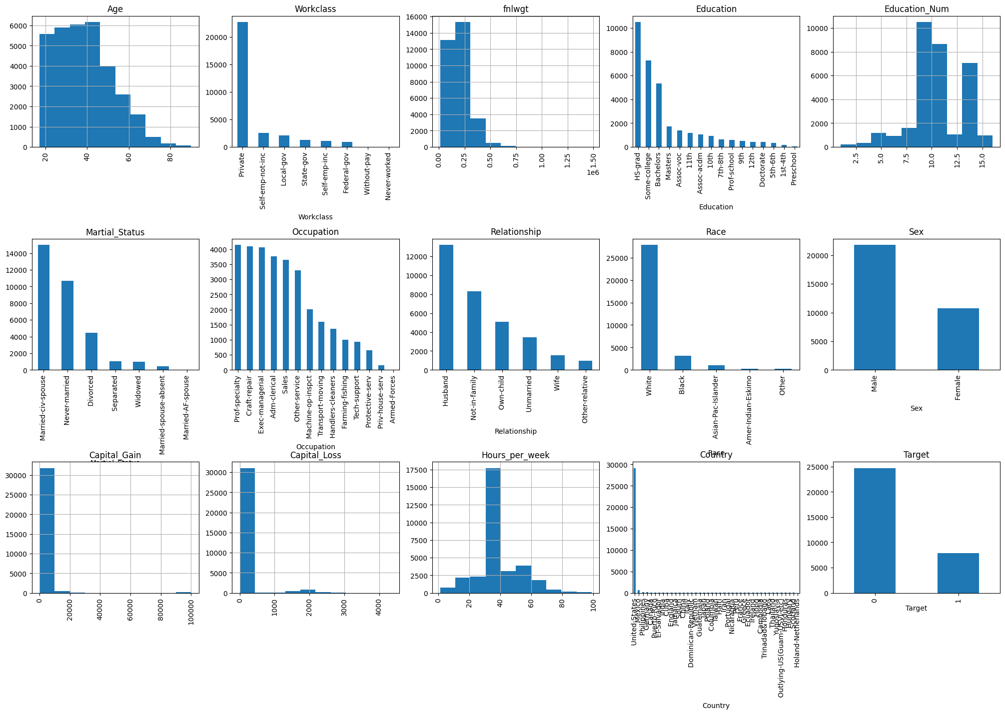
fig = plt.figure(figsize=(25, 15))
cols = 5
rows = int(data_train.shape[1] / cols)
for i, column in enumerate(data_train.columns):
    ax = fig.add_subplot(rows, cols, i + 1)
    ax.set_title(column)
    if data_train.dtypes[column] == object:
        data_train[column].value_counts().plot(kind="bar", axes=ax)
    else:
        data_train[column].hist(axes=ax)
        plt.xticks(rotation="vertical")
plt.subplots_adjust(hspace=0.7, wspace=0.2);
Checking data types
data_train.dtypes
Age                int64
Workclass         object
fnlwgt             int64
Education         object
Education_Num      int64
Martial_Status    object
Occupation        object
Relationship      object
Race              object
Sex               object
Capital_Gain       int64
Capital_Loss       int64
Hours_per_week     int64
Country           object
Target            object
dtype: object
data_test.dtypes
Age                object
Workclass          object
fnlwgt            float64
Education          object
Education_Num     float64
Martial_Status     object
Occupation         object
Relationship       object
Race               object
Sex                object
Capital_Gain      float64
Capital_Loss      float64
Hours_per_week    float64
Country            object
Target             object
dtype: object
As we see, in the test data, age is treated as type object. We need to fix this.
data_test["Age"] = data_test["Age"].astype(int)
Also we’ll cast all float features to int type to keep types consistent between our train and test data.
data_test["fnlwgt"] = data_test["fnlwgt"].astype(int)
data_test["Education_Num"] = data_test["Education_Num"].astype(int)
data_test["Capital_Gain"] = data_test["Capital_Gain"].astype(int)
data_test["Capital_Loss"] = data_test["Capital_Loss"].astype(int)
data_test["Hours_per_week"] = data_test["Hours_per_week"].astype(int)
Save targets separately.
y_train = data_train.pop('Target')
y_test = data_test.pop('Target')
Fill in missing data for continuous features with their median values, for categorical features with their mode.
# choose categorical and continuous features from data

categorical_columns = [
    c for c in data_train.columns if data_train[c].dtype.name == "object"
]
numerical_columns = [
    c for c in data_train.columns if data_train[c].dtype.name != "object"
]

print("categorical_columns:", categorical_columns)
print("numerical_columns:", numerical_columns)
categorical_columns: ['Workclass', 'Education', 'Martial_Status', 'Occupation', 'Relationship', 'Race', 'Sex', 'Country']
numerical_columns: ['Age', 'fnlwgt', 'Education_Num', 'Capital_Gain', 'Capital_Loss', 'Hours_per_week']
# we see some missing values
data_train.info()
<class 'pandas.core.frame.DataFrame'>
RangeIndex: 32561 entries, 0 to 32560
Data columns (total 14 columns):
 #   Column          Non-Null Count  Dtype
---  ------          --------------  -----
 0   Age             32561 non-null  int64
 1   Workclass       30725 non-null  object
 2   fnlwgt          32561 non-null  int64
 3   Education       32561 non-null  object
 4   Education_Num   32561 non-null  int64
 5   Martial_Status  32561 non-null  object
 6   Occupation      30718 non-null  object
 7   Relationship    32561 non-null  object
 8   Race            32561 non-null  object
 9   Sex             32561 non-null  object
 10  Capital_Gain    32561 non-null  int64
 11  Capital_Loss    32561 non-null  int64
 12  Hours_per_week  32561 non-null  int64
 13  Country         31978 non-null  object
dtypes: int64(6), object(8)
memory usage: 3.5+ MB
# fill missing data

for c in categorical_columns:
    data_train[c] = data_train[c].fillna(data_train[c].mode()[0])
    data_test[c] = data_test[c].fillna(data_train[c].mode()[0])

for c in numerical_columns:
    data_train[c] = data_train[c].fillna(data_train[c].median())
    data_test[c] = data_test[c].fillna(data_train[c].median())
# no more missing values
data_train.info()
<class 'pandas.core.frame.DataFrame'>
RangeIndex: 32561 entries, 0 to 32560
Data columns (total 14 columns):
 #   Column          Non-Null Count  Dtype
---  ------          --------------  -----
 0   Age             32561 non-null  int64
 1   Workclass       32561 non-null  object
 2   fnlwgt          32561 non-null  int64
 3   Education       32561 non-null  object
 4   Education_Num   32561 non-null  int64
 5   Martial_Status  32561 non-null  object
 6   Occupation      32561 non-null  object
 7   Relationship    32561 non-null  object
 8   Race            32561 non-null  object
 9   Sex             32561 non-null  object
 10  Capital_Gain    32561 non-null  int64
 11  Capital_Loss    32561 non-null  int64
 12  Hours_per_week  32561 non-null  int64
 13  Country         32561 non-null  object
dtypes: int64(6), object(8)
memory usage: 3.5+ MB
We’ll dummy code some categorical features: Workclass, Education, Martial_Status, Occupation, Relationship, Race, Sex, Country. It can be done via pandas method get_dummies
data_train = pd.concat(
    [data_train[numerical_columns], pd.get_dummies(data_train[categorical_columns])],
    axis=1,
)

data_test = pd.concat(
    [data_test[numerical_columns], pd.get_dummies(data_test[categorical_columns])],
    axis=1,
)
set(data_train.columns) - set(data_test.columns)
{'Country_ Holand-Netherlands'}
data_train.shape, data_test.shape
((32561, 105), (16281, 104))
There is no Holland in the test data. Create new zero-valued feature.
data_test["Country_ Holand-Netherlands"] = 0
set(data_train.columns) - set(data_test.columns)
set()
data_train.head(2)
| Age | fnlwgt | Education_Num | Capital_Gain | Capital_Loss | Hours_per_week | Workclass_ Federal-gov | Workclass_ Local-gov | Workclass_ Never-worked | Workclass_ Private | ... | Country_ Portugal | Country_ Puerto-Rico | Country_ Scotland | Country_ South | Country_ Taiwan | Country_ Thailand | Country_ Trinadad&Tobago | Country_ United-States | Country_ Vietnam | Country_ Yugoslavia | |
|---|---|---|---|---|---|---|---|---|---|---|---|---|---|---|---|---|---|---|---|---|---|
| 0 | 39 | 77516 | 13 | 2174 | 0 | 40 | False | False | False | False | ... | False | False | False | False | False | False | False | True | False | False |
| 1 | 50 | 83311 | 13 | 0 | 0 | 13 | False | False | False | False | ... | False | False | False | False | False | False | False | True | False | False |
2 rows × 105 columns
data_test.head(2)
| Age | fnlwgt | Education_Num | Capital_Gain | Capital_Loss | Hours_per_week | Workclass_ Federal-gov | Workclass_ Local-gov | Workclass_ Never-worked | Workclass_ Private | ... | Country_ Puerto-Rico | Country_ Scotland | Country_ South | Country_ Taiwan | Country_ Thailand | Country_ Trinadad&Tobago | Country_ United-States | Country_ Vietnam | Country_ Yugoslavia | Country_ Holand-Netherlands | |
|---|---|---|---|---|---|---|---|---|---|---|---|---|---|---|---|---|---|---|---|---|---|
| 1 | 25 | 226802 | 7 | 0 | 0 | 40 | False | False | False | True | ... | False | False | False | False | False | False | True | False | False | 0 |
| 2 | 38 | 89814 | 9 | 0 | 0 | 50 | False | False | False | True | ... | False | False | False | False | False | False | True | False | False | 0 |
2 rows × 105 columns
X_train = data_train
X_test = data_test
3.1 Decision tree without parameter tuning#
Train a decision tree (DecisionTreeClassifier) with a maximum depth of 3, and evaluate the accuracy metric on the test data. Use parameter random_state = 17 for results reproducibility.
# You code here (read-only in a JupyterBook, pls run jupyter-notebook to edit) (read-only in a JupyterBook, pls run jupyter-notebook to edit)
# tree =
# tree.fit
Make a prediction with the trained model on the test data.
# You code here (read-only in a JupyterBook, pls run jupyter-notebook to edit)
# tree_predictions = tree.predict
# You code here (read-only in a JupyterBook, pls run jupyter-notebook to edit)
# accuracy_score
6. What is the test set accuracy of a decision tree with maximum tree depth of 3 and random_state = 17?
3.2 Decision tree with parameter tuning#
Train a decision tree (DecisionTreeClassifier, random_state = 17). Find the optimal maximum depth using 5-fold cross-validation (GridSearchCV).
tree_params = {"max_depth": range(2, 11)}

locally_best_tree = GridSearchCV  # You code here (read-only in a JupyterBook, pls run jupyter-notebook to edit)

locally_best_tree.fit
# You code here (read-only in a JupyterBook, pls run jupyter-notebook to edit)
<function sklearn.model_selection._search.BaseSearchCV.fit(self, X, y=None, **params)>
Train a decision tree with maximum depth of 9 (it is the best max_depth in my case), and compute the test set accuracy. Use parameter random_state = 17 for reproducibility.
# You code here (read-only in a JupyterBook, pls run jupyter-notebook to edit)
# tuned_tree =
# tuned_tree.fit
# tuned_tree_predictions = tuned_tree.predict
# accuracy_score
7. What is the test set accuracy of a decision tree with maximum depth of 9 and random_state = 17?
3.3 (Optional) Random forest without parameter tuning#
Let’s take a sneak peek of upcoming lectures and try to use a random forest for our task. For now, you can imagine a random forest as a bunch of decision trees, trained on slightly different subsets of the training data.
Train a random forest (RandomForestClassifier). Set the number of trees to 100 and use random_state = 17.
# You code here (read-only in a JupyterBook, pls run jupyter-notebook to edit)
# rf =
# rf.fit # You code here (read-only in a JupyterBook, pls run jupyter-notebook to edit)
Make predictions for the test data and assess accuracy.
# You code here (read-only in a JupyterBook, pls run jupyter-notebook to edit)
3.4 (Optional) Random forest with parameter tuning#
Train a random forest (RandomForestClassifier). Tune the maximum depth and maximum number of features for each tree using GridSearchCV.
# forest_params = {'max_depth': range(10, 21),
#                 'max_features': range(5, 105, 20)}

# locally_best_forest = GridSearchCV # You code here (read-only in a JupyterBook, pls run jupyter-notebook to edit)

# locally_best_forest.fit # You code here (read-only in a JupyterBook, pls run jupyter-notebook to edit)
Make predictions for the test data and assess accuracy.
# You code here (read-only in a JupyterBook, pls run jupyter-notebook to edit)