Assignment #8 (demo). Implementation of online regressor. Solution

mlcourse.ai – Open Machine Learning Course
Author: Yury Kashnitsky. Translated by Sergey Oreshkov. This material is subject to the terms and conditions of the Creative Commons CC BY-NC-SA 4.0 license. Free use is permitted for any non-commercial purpose.

Same assignment as a Kaggle Notebook + solution.

Here we’ll implement a regressor trained with stochastic gradient descent (SGD). Fill in the missing code. If you do everything right, you’ll pass a simple embedded test.

Linear regression and Stochastic Gradient Descent

import numpy as np
import pandas as pd
from sklearn.base import BaseEstimator
from sklearn.metrics import log_loss, mean_squared_error, roc_auc_score
from sklearn.model_selection import train_test_split
from tqdm import tqdm

from matplotlib import pyplot as plt
%config InlineBackend.figure_format = 'retina'
import seaborn as sns
from sklearn.preprocessing import StandardScaler

Implement class SGDRegressor. Specification:

• class is inherited from sklearn.base.BaseEstimator

• constructor takes parameters eta – gradient step (\(10^{-3}\) by default) and n_epochs – dataset pass count (3 by default)

• constructor also creates mse_ and weights_ lists in order to track mean squared error and weight vector during gradient descent iterations

• Class has fit and predict methods

• The fit method takes matrix X and vector y (numpy.array objects) as parameters, appends column of ones to X on the left side, initializes weight vector w with zeros and then makes n_epochs iterations of weight updates (you may refer to this article for details), and for every iteration logs mean squared error and weight vector w in corresponding lists we created in the constructor.

• Additionally the fit method will create w_ variable to store weights which produce minimal mean squared error

• The fit method returns current instance of the SGDRegressor class, i.e. self

• The predict method takes X matrix, adds column of ones to the left side and returns prediction vector, using weight vector w_, created by the fit method.

class SGDRegressor(BaseEstimator):
    def __init__(self, eta=1e-3, n_epochs=3):
        self.eta = eta
        self.n_epochs = n_epochs
        self.mse_ = []
        self.weights_ = []

    def fit(self, X, y):
        X = np.hstack([np.ones([X.shape[0], 1]), X])

        w = np.zeros(X.shape[1])

        for it in tqdm(range(self.n_epochs)):
            for i in range(X.shape[0]):

                new_w = w.copy()
                new_w[0] += self.eta * (y[i] - w.dot(X[i, :]))
                for j in range(1, X.shape[1]):
                    new_w[j] += self.eta * (y[i] - w.dot(X[i, :])) * X[i, j]
                w = new_w.copy()

                self.weights_.append(w)
                self.mse_.append(mean_squared_error(y, X.dot(w)))

        self.w_ = self.weights_[np.argmin(self.mse_)]

        return self

    def predict(self, X):
        X = np.hstack([np.ones([X.shape[0], 1]), X])

        return X.dot(self.w_)

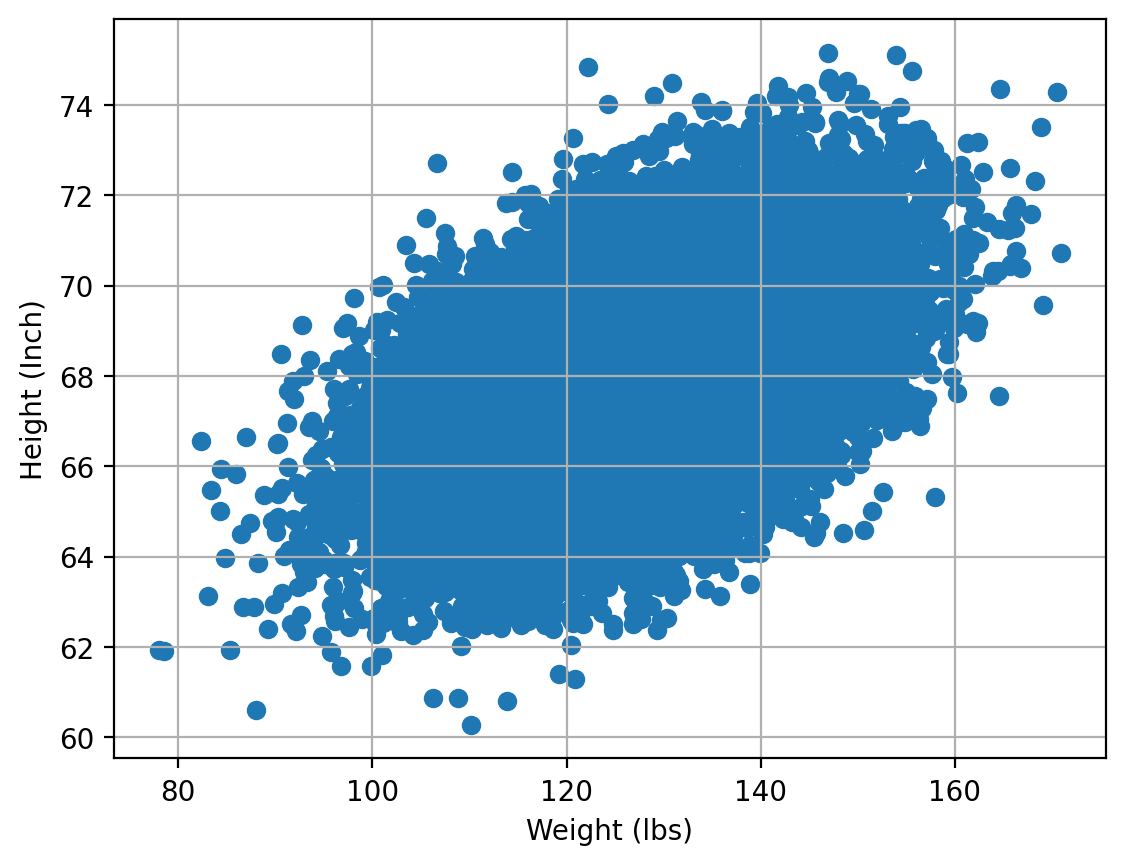
Let’s test out the algorithm on height/weight data. We will predict heights (in inches) based on weights (in lbs).

# for Jupyter-book, we copy data from GitHub, locally, to save Internet traffic,
# you can specify the data/ folder from the root of your cloned
# https://github.com/Yorko/mlcourse.ai repo, to save Internet traffic
DATA_PATH = "https://raw.githubusercontent.com/Yorko/mlcourse.ai/main/data/"

data_demo = pd.read_csv(DATA_PATH + "weights_heights.csv")

plt.scatter(data_demo["Weight"], data_demo["Height"])
plt.xlabel("Weight (lbs)")
plt.ylabel("Height (Inch)")
plt.grid();

X, y = data_demo["Weight"].values, data_demo["Height"].values

Perform train/test split and scale data.

X_train, X_valid, y_train, y_valid = train_test_split(
    X, y, test_size=0.3, random_state=17
)

scaler = StandardScaler()
X_train_scaled = scaler.fit_transform(X_train.reshape([-1, 1]))
X_valid_scaled = scaler.transform(X_valid.reshape([-1, 1]))

Train created SGDRegressor with (X_train_scaled, y_train) data. Leave default parameter values for now.

# you code here
sgd_reg = SGDRegressor()
sgd_reg.fit(X_train_scaled, y_train)

  0%|                                                                                                                                        | 0/3 [00:00<?, ?it/s]

 33%|██████████████████████████████████████████▋                                                                                     | 1/3 [00:05<00:11,  5.92s/it]

 67%|█████████████████████████████████████████████████████████████████████████████████████▎                                          | 2/3 [00:12<00:06,  6.03s/it]

100%|████████████████████████████████████████████████████████████████████████████████████████████████████████████████████████████████| 3/3 [00:18<00:00,  6.31s/it]

100%|████████████████████████████████████████████████████████████████████████████████████████████████████████████████████████████████| 3/3 [00:18<00:00,  6.23s/it]

SGDRegressor()

In a Jupyter environment, please rerun this cell to show the HTML representation or trust the notebook.
On GitHub, the HTML representation is unable to render, please try loading this page with nbviewer.org.

Draw a chart with training process – dependency of mean squared error from the i-th SGD iteration number.

# you code here
plt.plot(range(len(sgd_reg.mse_)), sgd_reg.mse_)
plt.xlabel("#updates")
plt.ylabel("MSE");

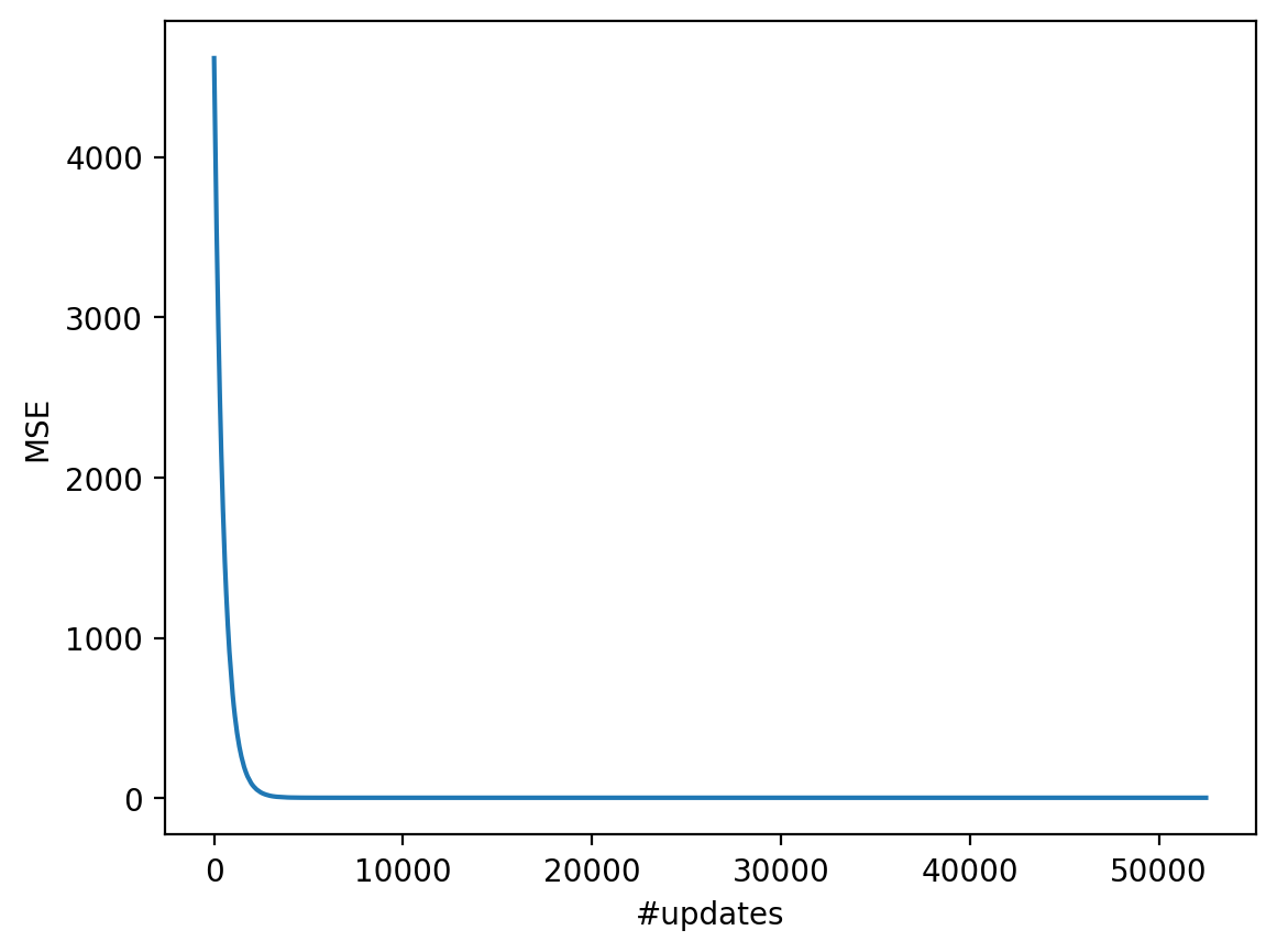
Print the minimal value of mean squared error and the best weights vector.

# you code here
np.min(sgd_reg.mse_), sgd_reg.w_

(2.7151352406643623, array([67.9898497 ,  0.94447605]))

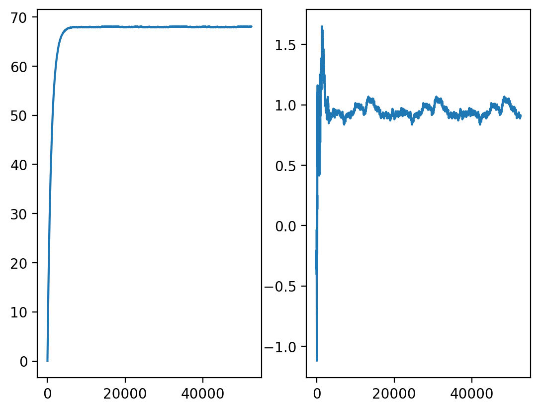
Draw chart of model weights (\(w_0\) and \(w_1\)) behavior during training.

# you code here
plt.subplot(121)
plt.plot(range(len(sgd_reg.weights_)), [w[0] for w in sgd_reg.weights_])
plt.subplot(122)
plt.plot(range(len(sgd_reg.weights_)), [w[1] for w in sgd_reg.weights_]);

Make a prediction for hold-out set (X_valid_scaled, y_valid) and check MSE value.

# you code here
sgd_holdout_mse = mean_squared_error(y_valid, sgd_reg.predict(X_valid_scaled))
sgd_holdout_mse

2.6708681207033784

Do the same thing for LinearRegression class from sklearn.linear_model. Evaluate MSE for hold-out set.

# you code here
from sklearn.linear_model import LinearRegression

lm = LinearRegression().fit(X_train_scaled, y_train)
print(lm.coef_, lm.intercept_)
linreg_holdout_mse = mean_squared_error(y_valid, lm.predict(X_valid_scaled))
linreg_holdout_mse

[0.94537278] 67.98930834742858

2.670830767667635

try:
    assert (sgd_holdout_mse - linreg_holdout_mse) < 1e-4
    print("Correct!")
except AssertionError:
    print(
        "Something's not good.\n Linreg's holdout MSE: {}"
        "\n SGD's holdout MSE: {}".format(linreg_holdout_mse, sgd_holdout_mse)
    )

Correct!