Assignment #9 (demo). Time series analysis. Solution#

Author: Mariya Mansurova, Analyst & developer in Yandex.Metrics team. Translated by Ivan Zakharov, ML enthusiast.
This material is subject to the terms and conditions of the Creative Commons CC BY-NC-SA 4.0 license. Free use is permitted for any non-commercial purpose.
Same assignment as a Kaggle Notebook + solution.
In this assignment, we are using Prophet and ARIMA to analyze the number of views for a Wikipedia page on Machine Learning.
Fill cells marked with “Your code here” and submit your answers to the questions through the web form.
import warnings

warnings.filterwarnings("ignore")
import os

import numpy as np
import pandas as pd
import requests
from plotly import __version__
from plotly import graph_objs as go
from plotly.offline import download_plotlyjs, init_notebook_mode, iplot, plot
from IPython.display import display, IFrame

print(__version__)  # need 1.9.0 or greater
init_notebook_mode(connected=True)
6.1.1
def plotly_df(df, title="", width=800, height=500):
    """Visualize all the dataframe columns as line plots."""
    common_kw = dict(x=df.index, mode="lines")
    data = [go.Scatter(y=df[c], name=c, **common_kw) for c in df.columns]
    layout = dict(title=title)
    fig = dict(data=data, layout=layout)

    # in a Jupyter Notebook, the following should work
    #iplot(fig, show_link=False)

    # in a Jupyter Book, we save a plot offline and then render it with IFrame
    plot_path = f"../../_static/plotly_htmls/{title}.html".replace(" ", "_")
    plot(fig, filename=plot_path, show_link=False, auto_open=False);
    display(IFrame(plot_path, width=width, height=height))
Data preparation#
# for Jupyter-book, we copy data from GitHub, locally, to save Internet traffic,
# you can specify the data/ folder from the root of your cloned
# https://github.com/Yorko/mlcourse.ai repo, to save Internet traffic
DATA_PATH = "https://raw.githubusercontent.com/Yorko/mlcourse.ai/main/data/"
df = pd.read_csv(DATA_PATH + "wiki_machine_learning.csv", sep=" ")
df = df[df["count"] != 0]
df.head()
| date | count | lang | page | rank | month | title | |
|---|---|---|---|---|---|---|---|
| 81 | 2015-01-01 | 1414 | en | Machine_learning | 8708 | 201501 | Machine_learning |
| 80 | 2015-01-02 | 1920 | en | Machine_learning | 8708 | 201501 | Machine_learning |
| 79 | 2015-01-03 | 1338 | en | Machine_learning | 8708 | 201501 | Machine_learning |
| 78 | 2015-01-04 | 1404 | en | Machine_learning | 8708 | 201501 | Machine_learning |
| 77 | 2015-01-05 | 2264 | en | Machine_learning | 8708 | 201501 | Machine_learning |
df.shape
(383, 7)
Predicting with FB Prophet#
We will train on the first 5 months and predict the number of trips for June.
df.date = pd.to_datetime(df.date)
plotly_df(df=df.set_index("date")[["count"]], title="assign9_plot")
from prophet import Prophet
predictions = 30

df = df[["date", "count"]]
df.columns = ["ds", "y"]
df.tail()
| ds | y | |
|---|---|---|
| 382 | 2016-01-16 | 1644 |
| 381 | 2016-01-17 | 1836 |
| 376 | 2016-01-18 | 2983 |
| 375 | 2016-01-19 | 3389 |
| 372 | 2016-01-20 | 3559 |
train_df = df[:-predictions].copy()
m = Prophet()
m.fit(train_df)
10:43:02 - cmdstanpy - INFO - Chain [1] start processing
10:43:02 - cmdstanpy - INFO - Chain [1] done processing
<prophet.forecaster.Prophet at 0x158db52b0>
future = m.make_future_dataframe(periods=predictions)
future.tail()
| ds | |
|---|---|
| 378 | 2016-01-16 |
| 379 | 2016-01-17 |
| 380 | 2016-01-18 |
| 381 | 2016-01-19 |
| 382 | 2016-01-20 |
forecast = m.predict(future)
forecast.tail()
| ds | trend | yhat_lower | yhat_upper | trend_lower | trend_upper | additive_terms | additive_terms_lower | additive_terms_upper | weekly | weekly_lower | weekly_upper | multiplicative_terms | multiplicative_terms_lower | multiplicative_terms_upper | yhat | |
|---|---|---|---|---|---|---|---|---|---|---|---|---|---|---|---|---|
| 378 | 2016-01-16 | 2977.168399 | 1701.742621 | 2496.526531 | 2956.300983 | 2998.268438 | -861.727923 | -861.727923 | -861.727923 | -861.727923 | -861.727923 | -861.727923 | 0.0 | 0.0 | 0.0 | 2115.440476 |
| 379 | 2016-01-17 | 2982.524268 | 1865.316607 | 2664.209429 | 2960.282415 | 3005.035825 | -720.760235 | -720.760235 | -720.760235 | -720.760235 | -720.760235 | -720.760235 | 0.0 | 0.0 | 0.0 | 2261.764034 |
| 380 | 2016-01-18 | 2987.880138 | 2880.057162 | 3672.672982 | 2964.704694 | 3011.561143 | 281.393573 | 281.393573 | 281.393573 | 281.393573 | 281.393573 | 281.393573 | 0.0 | 0.0 | 0.0 | 3269.273711 |
| 381 | 2016-01-19 | 2993.236008 | 3107.390591 | 3921.247857 | 2969.107310 | 3018.597086 | 541.459498 | 541.459498 | 541.459498 | 541.459498 | 541.459498 | 541.459498 | 0.0 | 0.0 | 0.0 | 3534.695506 |
| 382 | 2016-01-20 | 2998.591877 | 2992.940380 | 3821.484388 | 2972.969987 | 3025.147112 | 425.524867 | 425.524867 | 425.524867 | 425.524867 | 425.524867 | 425.524867 | 0.0 | 0.0 | 0.0 | 3424.116744 |
Question 1: What is the prediction of the number of views of the wiki page on January 20? Round to the nearest integer.
4947
3426 [+]
5229
2744
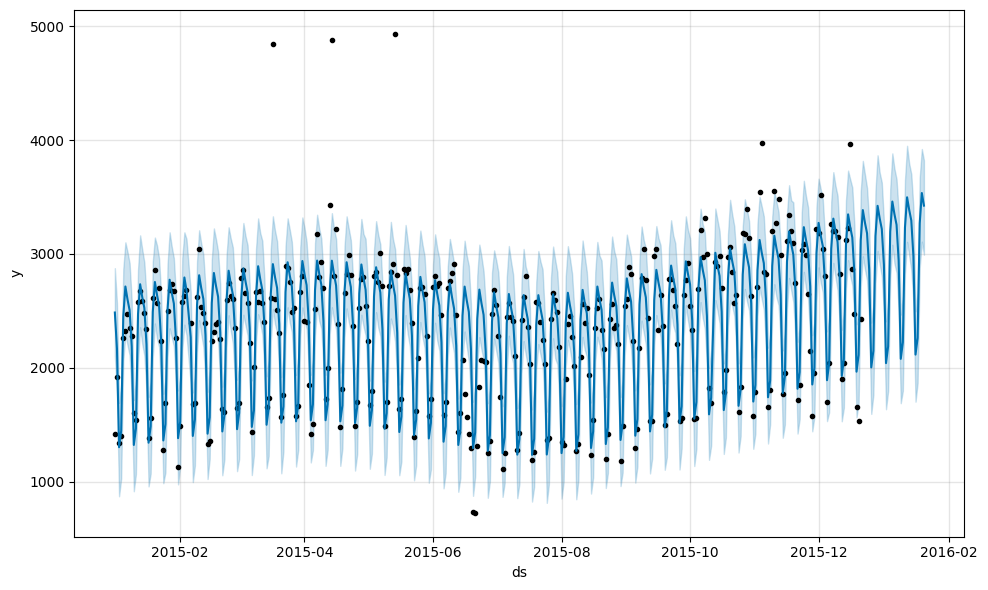
m.plot(forecast)
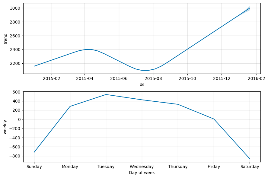
m.plot_components(forecast)
cmp_df = forecast.set_index("ds")[["yhat", "yhat_lower", "yhat_upper"]].join(
    df.set_index("ds")
)
cmp_df["e"] = cmp_df["y"] - cmp_df["yhat"]
cmp_df["p"] = 100 * cmp_df["e"] / cmp_df["y"]
print("MAPE = ", round(np.mean(abs(cmp_df[-predictions:]["p"])), 2))
print("MAE = ", round(np.mean(abs(cmp_df[-predictions:]["e"])), 2))
MAPE =  34.43
MAE =  598.39
Estimate the quality of the prediction with the last 30 points.
Question 2: What is MAPE equal to?
34.5 [+]
42.42
5.39
65.91
Question 3: What is MAE equal to?
355
4007
600 [+]
903
Predicting with ARIMA#
%matplotlib inline
import matplotlib.pyplot as plt
import statsmodels.api as sm
from scipy import stats

plt.rcParams["figure.figsize"] = (15, 10)
Question 4: Let’s verify the stationarity of the series using the Dickey-Fuller test. Is the series stationary? What is the p-value?
Series is stationary, p_value = 0.107
Series is not stationary, p_value = 0.107 [+]
Series is stationary, p_value = 0.001
Series is not stationary, p_value = 0.001
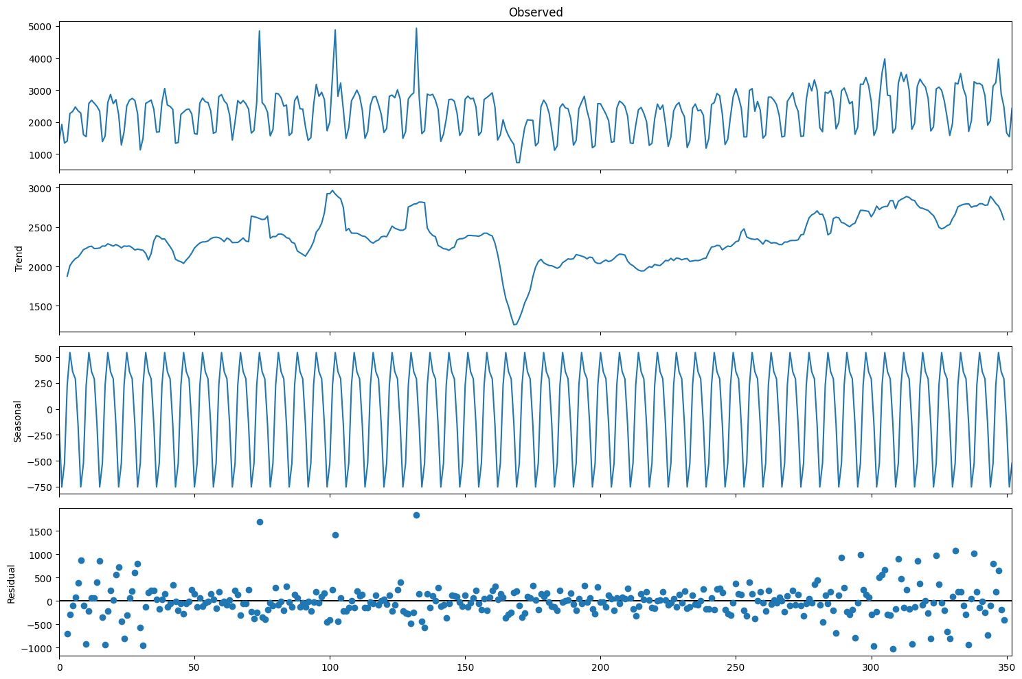
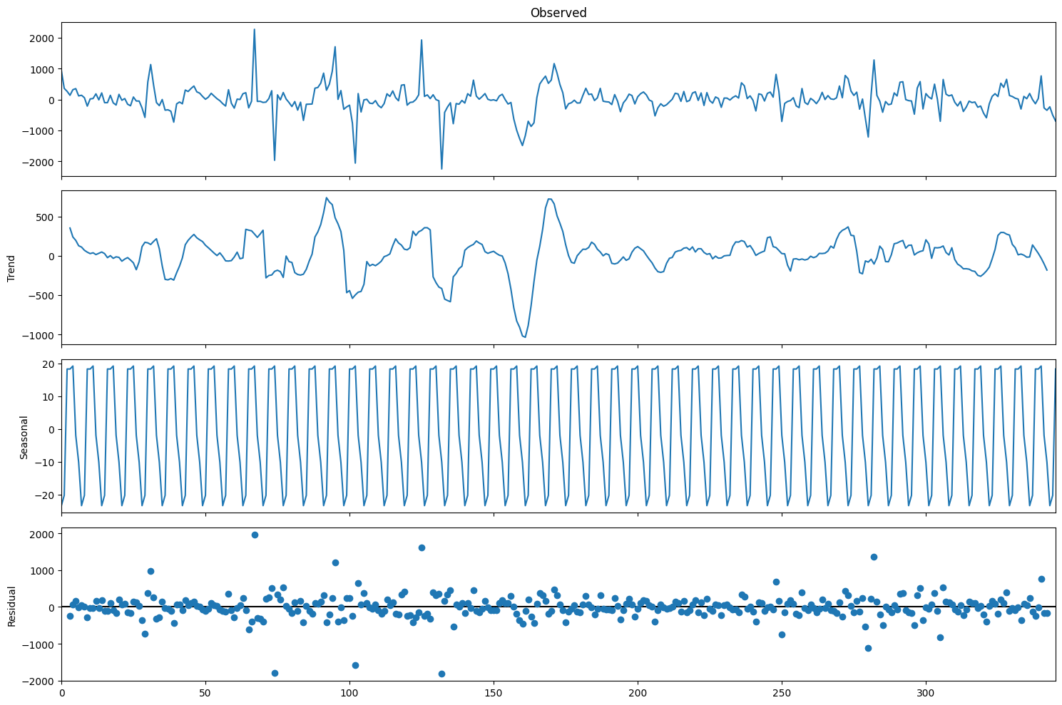
sm.tsa.seasonal_decompose(train_df["y"].values, period=7).plot()
print("Dickey-Fuller test: p=%f" % sm.tsa.stattools.adfuller(train_df["y"])[1])
Dickey-Fuller test: p=0.107392
But the seasonally differentiated series will already be stationary.
train_df.set_index("ds", inplace=True)
train_df["y_diff"] = train_df.y - train_df.y.shift(7)
sm.tsa.seasonal_decompose(train_df.y_diff[7:].values, period=7).plot()
print("Dickey-Fuller test: p=%f" % sm.tsa.stattools.adfuller(train_df.y_diff[8:])[1])
Dickey-Fuller test: p=0.000000
ax = plt.subplot(211)
sm.graphics.tsa.plot_acf(train_df.y_diff[13:].values.squeeze(), lags=48, ax=ax)

ax = plt.subplot(212)
sm.graphics.tsa.plot_pacf(train_df.y_diff[13:].values.squeeze(), lags=48, ax=ax)
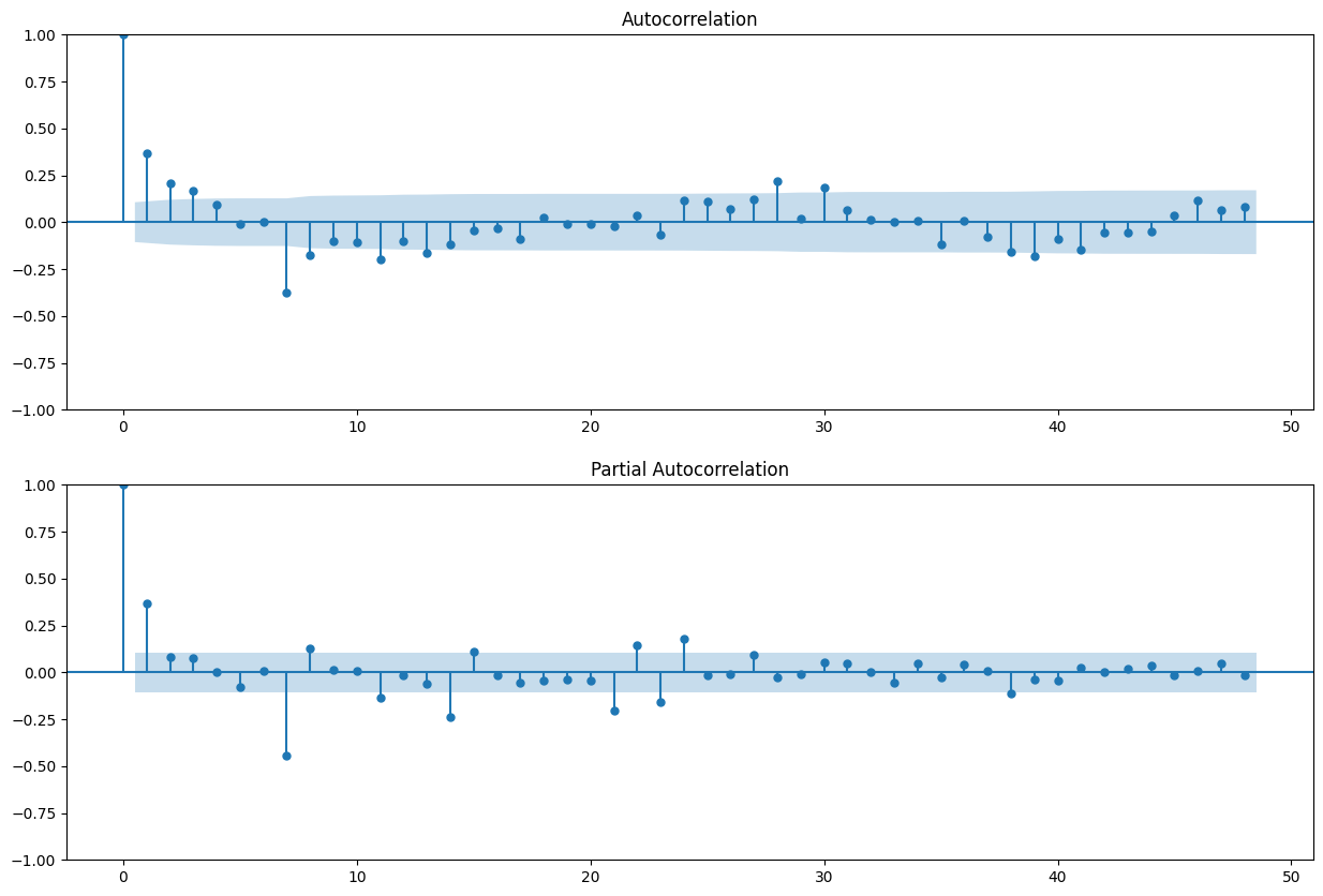
Initial values:
Q = 1
q = 3
P = 3
p = 1
ps = range(0, 2)
ds = range(0, 2)
qs = range(0, 4)
Ps = range(0, 4)
Ds = range(0, 3)
Qs = range(0, 2)
from itertools import product

parameters = product(ps, ds, qs, Ps, Ds, Qs)
parameters_list = list(parameters)
len(parameters_list)
384
%%time
import warnings

from tqdm.notebook import tqdm

results1 = []
best_aic = float("inf")
warnings.filterwarnings("ignore")

for param in tqdm(parameters_list):
    # try except is necessary, because on some sets of parameters the model can not be trained
    try:
        model = sm.tsa.statespace.SARIMAX(
            train_df["y"],
            order=(param[0], param[1], param[2]),
            seasonal_order=(param[3], param[4], param[5], 7),
            # train the model as is even if that would lead to a non-stationary / non-invertible model
            # see https://github.com/statsmodels/statsmodels/issues/6225 for details
        ).fit(disp=-1)

    except (ValueError, np.linalg.LinAlgError):
        continue

    aic = model.aic
    # save the best model, aic, parameters
    if aic < best_aic:
        best_model = model
        best_aic = aic
        best_param = param
    results1.append([param, model.aic])
CPU times: user 2min 27s, sys: 1.62 s, total: 2min 28s
Wall time: 2min 30s
result_table1 = pd.DataFrame(results1)
result_table1.columns = ["parameters", "aic"]
print(result_table1.sort_values(by="aic", ascending=True).head())
             parameters          aic
66   (0, 0, 2, 3, 0, 1)    14.000000
328  (1, 1, 1, 3, 0, 1)    14.000000
89   (0, 0, 3, 3, 0, 0)    14.000000
165  (0, 1, 2, 3, 2, 1)  4961.632632
332  (1, 1, 1, 3, 2, 1)  4962.841640
If we consider the variants proposed in the form:
result_table1[
    result_table1["parameters"].isin(
        [(1, 0, 2, 3, 1, 0), (1, 1, 2, 3, 2, 1), (1, 1, 2, 3, 1, 1), (1, 0, 2, 3, 0, 0)]
    )
].sort_values(by="aic")
| parameters | aic | |
|---|---|---|
| 356 | (1, 1, 2, 3, 2, 1) | 4989.004019 |
| 354 | (1, 1, 2, 3, 1, 1) | 5019.555903 |
| 257 | (1, 0, 2, 3, 1, 0) | 5022.312524 |
| 255 | (1, 0, 2, 3, 0, 0) | 5174.678617 |
Now do the same, but for the series with Box-Cox transformation.
import scipy.stats

train_df["y_box"], lmbda = scipy.stats.boxcox(train_df["y"])
print("The optimal Box-Cox transformation parameter: %f" % lmbda)
The optimal Box-Cox transformation parameter: 0.732841
results2 = []
best_aic = float("inf")

for param in tqdm(parameters_list):
    # try except is necessary, because on some sets of parameters the model can not be trained
    try:
        model = sm.tsa.statespace.SARIMAX(
            train_df["y_box"],
            order=(param[0], param[1], param[2]),
            seasonal_order=(param[3], param[4], param[5], 7),
            # train the model as is even if that would lead to a non-stationary / non-invertible model
            # see https://github.com/statsmodels/statsmodels/issues/6225 for details
            enforce_stationarity=False,
            enforce_invertibility=False
        ).fit(disp=-1)

    except (ValueError, np.linalg.LinAlgError):
        continue

    aic = model.aic
    # save the best model, aic, parameters
    if aic < best_aic:
        best_model = model
        best_aic = aic
        best_param = param
    results2.append([param, model.aic])

warnings.filterwarnings("default")
result_table2 = pd.DataFrame(results2)
result_table2.columns = ["parameters", "aic"]
print(result_table2.sort_values(by="aic", ascending=True).head())
             parameters          aic
263  (1, 0, 2, 3, 2, 1)  3292.640166
287  (1, 0, 3, 3, 2, 1)  3294.134383
215  (1, 0, 0, 3, 2, 1)  3294.194179
239  (1, 0, 1, 3, 2, 1)  3296.022150
383  (1, 1, 3, 3, 2, 1)  3296.540788
If we consider the variants proposed in the form:
result_table2[
    result_table2["parameters"].isin(
        [(1, 0, 2, 3, 1, 0), (1, 1, 2, 3, 2, 1), (1, 1, 2, 3, 1, 1), (1, 0, 2, 3, 0, 0)]
    )
].sort_values(by="aic")
| parameters | aic | |
|---|---|---|
| 359 | (1, 1, 2, 3, 2, 1) | 3326.066533 |
| 357 | (1, 1, 2, 3, 1, 1) | 3335.179337 |
| 260 | (1, 0, 2, 3, 1, 0) | 3335.555977 |
| 258 | (1, 0, 2, 3, 0, 0) | 3511.184072 |
Next, we turn to the construction of the SARIMAX model (sm.tsa.statespace.SARIMAX).
Question 5: What parameters are the best for the model according to the AIC criterion?
D = 1, d = 0, Q = 0, q = 2, P = 3, p = 1
D = 2, d = 1, Q = 1, q = 2, P = 3, p = 1 [+]
D = 1, d = 1, Q = 1, q = 2, P = 3, p = 1
D = 0, d = 0, Q = 0, q = 2, P = 3, p = 1
Let’s look at the forecast of the best AIC model.
Note: any AIC below 3000 is suspicious, probably caused by non-convergence with MLE optimization, we’ll pick the 3rd-best model in terms of AIC to visualize predictions.
best_model = sm.tsa.statespace.SARIMAX(
    train_df["y_box"],
    order=(1, 0, 2),
    seasonal_order=(3, 2, 1, 7),
    enforce_stationarity=False,
    enforce_invertibility=False
).fit(disp=-1)
/Users/kashnitsky/Documents/misc/mlcourse.ai/.venv/lib/python3.13/site-packages/statsmodels/tsa/base/tsa_model.py:473: ValueWarning:

A date index has been provided, but it has no associated frequency information and so will be ignored when e.g. forecasting.
print(best_model.summary())
                                      SARIMAX Results
===========================================================================================
Dep. Variable:                               y_box   No. Observations:                  353
Model:             SARIMAX(1, 0, 2)x(3, 2, [1], 7)   Log Likelihood               -1638.320
Date:                             Thu, 15 Jan 2026   AIC                           3292.640
Time:                                     10:47:24   BIC                           3322.711
Sample:                                          0   HQIC                          3304.652
                                             - 353
Covariance Type:                               opg
==============================================================================
                 coef    std err          z      P>|z|      [0.025      0.975]
------------------------------------------------------------------------------
ar.L1          0.8153      0.115      7.091      0.000       0.590       1.041
ma.L1         -0.3308      0.124     -2.671      0.008      -0.574      -0.088
ma.L2         -0.2102      0.096     -2.200      0.028      -0.397      -0.023
ar.S.L7       -0.6861      0.041    -16.644      0.000      -0.767      -0.605
ar.S.L14      -0.4749      0.059     -7.990      0.000      -0.591      -0.358
ar.S.L21      -0.2977      0.044     -6.809      0.000      -0.383      -0.212
ma.S.L7       -0.9706      0.059    -16.572      0.000      -1.085      -0.856
sigma2      1705.7076    106.729     15.982      0.000    1496.523    1914.892
===================================================================================
Ljung-Box (L1) (Q):                   0.04   Jarque-Bera (JB):               470.60
Prob(Q):                              0.85   Prob(JB):                         0.00
Heteroskedasticity (H):               0.61   Skew:                             0.94
Prob(H) (two-sided):                  0.01   Kurtosis:                         8.67
===================================================================================

Warnings:
[1] Covariance matrix calculated using the outer product of gradients (complex-step).
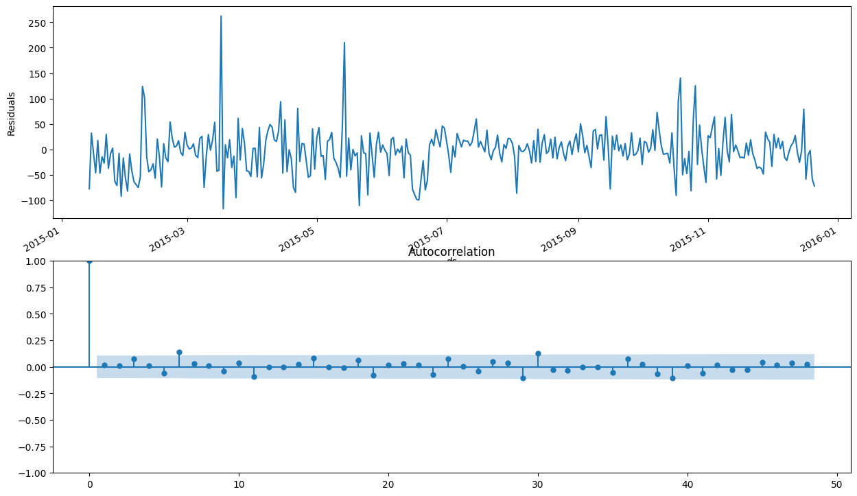
plt.subplot(211)
best_model.resid[13:].plot()
plt.ylabel(u"Residuals")

ax = plt.subplot(212)
sm.graphics.tsa.plot_acf(best_model.resid[13:].values.squeeze(), lags=48, ax=ax)

print("Student's test: p=%f" % stats.ttest_1samp(best_model.resid[13:], 0)[1])
print("Dickey-Fuller test: p=%f" % sm.tsa.stattools.adfuller(best_model.resid[13:])[1])
Student's test: p=0.293588
Dickey-Fuller test: p=0.000000
def invboxcox(y, lmbda):
    # reverse Box Cox transformation
    if lmbda == 0:
        return np.exp(y)
    else:
        return np.exp(np.log(lmbda * y + 1) / lmbda)
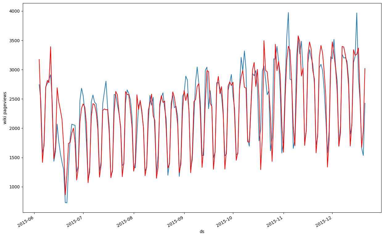
train_df["arima_model"] = invboxcox(best_model.fittedvalues, lmbda)

train_df.y.tail(200).plot()
train_df.arima_model[13:].tail(200).plot(color="r")
plt.ylabel("wiki pageviews");