Topic 4. Linear Classification and Regression#
Part 1. Ordinary Least Squares#

Author: Pavel Nesterov. Translated and edited by Christina Butsko, Yury Kashnitsky, Nerses Bagiyan, Yulia Klimushina, and Yuanyuan Pao. This material is subject to the terms and conditions of the Creative Commons CC BY-NC-SA 4.0 license. Free use is permitted for any non-commercial purpose.
Article outline#
1. Introduction#
We will start studying linear models with linear regression. First of all, you must specify a model that relates the dependent variable \(y\) to the explanatory factors (or features); for linear models, the dependency function will take the following form: \(\large y = w_0 + \sum_{i=1}^m w_i x_i\), where \(m\) is the number of features. If we add a fictitious dimension \(x_0 = 1\) (called bias or intercept term) for each observation, then the linear form can be rewritten in a slightly more compact way by pulling the absolute term \(w_0\) into the sum: \(\large y = \sum_{i=0}^m w_i x_i = \textbf{w}^\text{T} \textbf{x}\). If we have a matrix of \(n\) observations, where the rows are observations from a data set, we need to add a single column of ones on the left. We define the model as follows:
where
\(\textbf w \in \mathbb{R}^{m+1}\) – is an \((m+1) \times 1\) column-vector of the model parameters (in machine learning, these parameters are often referred to as weights);
\(\textbf X \in \mathbb{R}^{n \times (m+1)}\) – is an \(n \times (m+1)\) matrix of observations and their features, (including the fictitious column on the left) with full column rank: \(\text{rank}\left(\textbf X\right) = m + 1 \);
\(\epsilon \in \mathbb{R}^n\) – is an \(n \times 1\) random column-vector, referred to as error or noise;
\(\textbf y \in \mathbb{R}^n\) – is an \(n \times 1\) column-vector - the dependent (or target) variable.
We can also write this expression out for each observation
We will apply the following restrictions to the set of random errors \(\epsilon_i\) (see Gauss-Markov theorem for deeper statistical motivation):
expectation of all random errors is zero: \(\forall i: \mathbb{E}\left[\epsilon_i\right] = 0 \);
all random errors have the same finite variance, this property is called homoscedasticity: \(\forall i: \text{Var}\left(\epsilon_i\right) = \sigma^2 < \infty \);
random errors are uncorrelated: \(\forall i \neq j: \text{Cov}\left(\epsilon_i, \epsilon_j\right) = 0 \).
Estimator \(\widehat{w}_i \) of weights \(w_i \) is called linear if
where \(\forall\ k\ \), \(\omega_{ki} \) depend only on the samples from \(\textbf X\), but not on \(\textbf w\) - we don’t know the true coefficients \(w_i\) (that’s why we try to estimate them with the given data). Since the solution for finding the optimal weights is a linear estimator, the model is called linear regression.
Disclaimer: at this point, it’s time to say that we don’t plan to squeeze a whole statistics course into one article, so we try to provide the general idea of the math behind OLS.
Let’s introduce one more definition. Estimator \(\widehat{w}_i \) is called unbiased when its expectation is equal to the real but unknown value of the estimated parameter:
One of the ways to calculate those weights is with the ordinary least squares method (OLS), which minimizes the mean squared error between the actual value of the dependent variable and the predicted value given by the model:
To solve this optimization problem, we need to calculate derivatives with respect to the model parameters. We set them to zero and solve the resulting equation for \(\textbf w\) (matrix differentiation may seem difficult; try to do it in terms of sums to be sure of the answer).
Small CheatSheet on matrix derivatives (click the triangle to extend)
What we get is:
Bearing in mind all the definitions and conditions described above, we can say that, based on the Gauss–Markov theorem, OLS estimators of the model parameters are optimal among all linear and unbiased estimators, i.e., they give the lowest variance.
2. Maximum Likelihood Estimation#
One could ask why we choose to minimize the mean square error instead of something else? After all, one can minimize the mean absolute value of the residual. The only thing that will happen, if we change the minimized value, is that we will exceed the Gauss-Markov theorem conditions, and our estimates will therefore cease to be the optimal over the linear and unbiased ones.
Before we continue, let’s digress to illustrate maximum likelihood estimation with a simple example.
Many people probably remember the formula of ethyl alcohol, so I decided to do an experiment to determine whether people remember a simpler formula for methanol: \(CH_3OH\). We surveyed 400 people to find that only 117 people remembered the formula. Then, it is reasonable to assume that the probability that the next respondent knows the formula of methyl alcohol is \(\frac{117}{400} \approx 29\%\). Let’s show that this intuitive assessment is not only good but also a maximum likelihood estimate. Where does this estimate come from? Recall the definition of the Bernoulli distribution: a random variable has a Bernoulli distribution if it takes only two values (\(1\) and \(0\) with probability \(\theta\) and \(1 - \theta\), respectively) and has the following probability distribution function:
This distribution is exactly what we need, and the distribution parameter \(\theta\) is the estimate of the probability that a person knows the formula of methyl alcohol. In our \(400\) independent experiments, let’s denote their outcomes as \(\textbf{x} = \left(x_1, x_2, \ldots, x_{400}\right)\). Let’s write down the likelihood of our data (observations), i.e. the probability of observing exactly these 117 realizations of the random variable \(x = 1\) and 283 realizations of \(x = 0\):
Next, we will maximize the expression with respect to \(\theta\). Most often this is not done with the likelihood \(p(\textbf{x}; \theta)\) but with its logarithm (the monotonic transformation does not change the solution but simplifies calculation greatly):
Now, we want to find such a value of \(\theta\) that will maximize the likelihood. For this purpose, we’ll take the derivative with respect to \(\theta\), set it to zero, and solve the resulting equation:
It turns out that our intuitive assessment is exactly the maximum likelihood estimate. Now let us apply the same reasoning to the linear regression problem and try to find out what lies beyond the mean squared error. To do this, we’ll need to look at linear regression from a probabilistic perspective. Our model naturally remains the same:
but let us now assume that the random errors follow a centered Normal distribution (beware, it’s an additional assumption, it’s not a prerequisite of a Gauss-Markov theorem):
Let’s rewrite the model from a new perspective:
Since the examples are taken independently (uncorrelated errors is one of the conditions of the Gauss-Markov theorem), the full likelihood of the data will look like a product of the density functions \(p\left(y_i\right)\). Let’s consider the log-likelihood, which allows us to switch products to sums:
We want to find the maximum likelihood hypothesis i.e. we need to maximize the expression \(p\left(\textbf{y} \mid \textbf X; \textbf{w}\right)\) to get \(\textbf{w}_{\text{ML}}\), which is the same as maximizing its logarithm. Note that, while maximizing the function over some parameter, you can throw away all the members that do not depend on this parameter:
Thus, we have seen that the maximization of the likelihood of data is the same as the minimization of the mean squared error (given the above assumptions). It turns out that such a cost function is a consequence of the fact that the errors are distributed normally.
3. Bias-Variance Decomposition#
Let’s talk a little about the error properties of linear regression prediction (in fact, this discussion is valid for all machine learning algorithms). We just covered the following:
true value of the target variable is the sum of a deterministic function \(f\left(\textbf{x}\right)\) and random error \(\epsilon\): \(y = f\left(\textbf{x}\right) + \epsilon\);
error is normally distributed with zero mean and some variance: \(\epsilon \sim \mathcal{N}\left(0, \sigma^2\right)\);
true value of the target variable is also normally distributed: \(y \sim \mathcal{N}\left(f\left(\textbf{x}\right), \sigma^2\right)\);
we try to approximate a deterministic but unknown function \(f\left(\textbf{x}\right)\) using a linear function of the covariates \(\widehat{f}\left(\textbf{x}\right)\), which, in turn, is a point estimate of the function \(f\) in function space (specifically, the family of linear functions that we have limited our space to), i.e. a random variable that has mean and variance.
So, the error at the point \(\textbf{x}\) decomposes as follows:
For clarity, we will omit the notation of the argument of the functions. Let’s consider each member separately. The first two are easily decomposed according to the formula \(\text{Var}\left(z\right) = \mathbb{E}\left[z^2\right] - \mathbb{E}\left[z\right]^2\):
Note that:
And finally, we get to the last term in the sum. Recall that the error and the target variable are independent of each other:
Finally, let’s bring this all together:
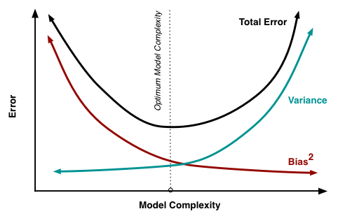
With that, we have reached our ultimate goal – the last formula tells us that the forecast error of any model of type \(y = f\left(\textbf{x}\right) + \epsilon\) is composed of:
squared bias: \(\text{Bias}\left(\widehat{f}\right)\) is the average error for all sets of data;
variance: \(\text{Var}\left(\widehat{f}\right)\) is error variability, or by how much error will vary if we train the model on different sets of data;
irremovable error: \(\sigma^2\).
While we cannot do anything with the \(\sigma^2\) term, we can influence the first two. Ideally, we’d like to eliminate both of these terms (upper left square of the picture), but, in practice, it is often necessary to balance between the biased and unstable estimates (high variance).
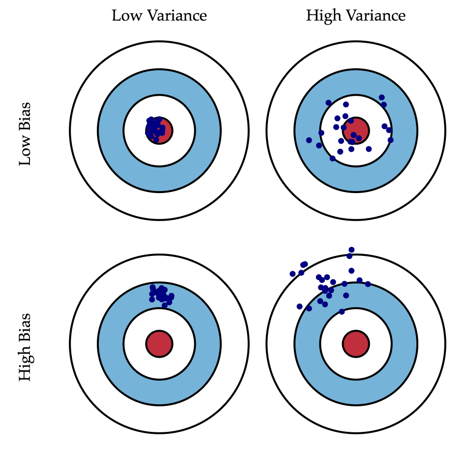
Generally, as the model becomes more computational (e.g. when the number of free parameters grows), the variance (dispersion) of the estimate also increases, but bias decreases. Due to the fact that the training set is memorized completely instead of generalizing, small changes lead to unexpected results (overfitting). On the other side, if the model is too weak, it will not be able to learn the pattern, resulting in learning something different that is offset with respect to the right solution.
The Gauss-Markov theorem asserts that the OLS estimator of parameters of the linear model is the best for the class of linear unbiased estimators. This means that if there exists any other unbiased model \(g\), from the same class of linear models, we can be sure that \(Var\left(\widehat{f}\right) \leq Var\left(g\right)\).
4. Regularization of Linear Regression#
There are situations where we might intentionally increase the bias of the model for the sake of stability i.e. to reduce the variance of the model \(\text{Var}\left(\widehat{f}\right)\). One of the conditions of the Gauss-Markov theorem is the full column rank of matrix \(\textbf{X}\). Otherwise, the OLS solution \(\textbf{w} = \left(\textbf{X}^\text{T} \textbf{X}\right)^{-1} \textbf{X}^\text{T} \textbf{y}\) does not exist since the inverse matrix \(\left(\textbf{X}^\text{T} \textbf{X}\right)^{-1}\) does not exist. In other words, matrix \(\textbf{X}^\text{T} \textbf{X}\) will be singular or degenerate. This problem is called an ill-posed problem. Problems like this must be corrected, namely, matrix \(\textbf{X}^\text{T} \textbf{X}\) needs to become non-degenerate, or regular (which is why this process is called regularization). Often we observe the so-called multicollinearity in the data: when two or more features are strongly correlated, it is manifested in the matrix \(\textbf{X}\) in the form of “almost” linear dependence between the columns. For example, in the problem of predicting house prices by their parameters, attributes “area with balcony” and “area without balcony” will have an “almost” linear relationship. Formally, matrix \(\textbf{X}^\text{T} \textbf{X}\) for such data is reversible, but, due to multicollinearity, some of its eigenvalues will be close to zero. In the inverse matrix \(\textbf{X}^\text{T} \textbf{X}\), some extremely large eigenvalues will appear, as eigenvalues of the inverse matrix are \(\frac{1}{\lambda_i}\). The result of this vacillation of eigenvalues is an unstable estimate of model parameters, i.e. adding a new set of observations to the training data will lead to a completely different solution. One method of regularization is Tikhonov regularization, which generally looks like the addition of a new term to the mean squared error:
The Tikhonov matrix is often expressed as the product of a number by the identity matrix: \(\Gamma = \frac{\lambda}{2} E\). In this case, the problem of minimizing the mean squared error becomes a problem with a restriction on the \(L_2\) norm. If we differentiate the new cost function with respect to the model parameters, set the resulting function to zero, and rearrange for \(\textbf{w}\), we get the exact solution of the problem.
This type of regression is called ridge regression. The ridge is the diagonal matrix that we add to the \(\textbf{X}^\text{T} \textbf{X}\) matrix to ensure that we get a regular matrix as a result.

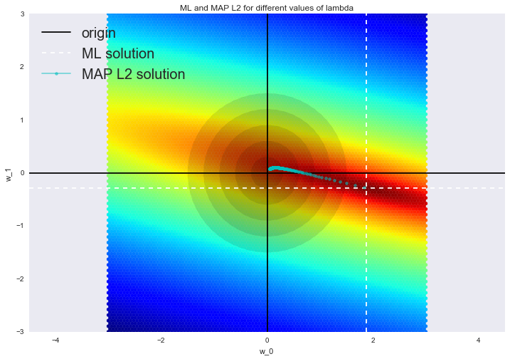
Such a solution reduces dispersion but becomes biased because the norm of the vector of parameters is also minimized, which makes the solution shift towards zero. On the figure below, the OLS solution is at the intersection of the white dotted lines. Blue dots represent different solutions of ridge regression. It can be seen that by increasing the regularization parameter \(\lambda\), we shift the solution towards zero.
5. Useful resources#
Medium “story” based on this notebook
Main course site, course repo, and YouTube channel
Course materials as a Kaggle Dataset
If you read Russian: an article on Habrahabr with ~ the same material. And a lecture on YouTube
A nice and concise overview of linear models is given in the book “Deep Learning” (I. Goodfellow, Y. Bengio, and A. Courville).
Linear models are covered practically in every ML book. We recommend “Pattern Recognition and Machine Learning” (C. Bishop) and “Machine Learning: A Probabilistic Perspective” (K. Murphy).
If you prefer a thorough overview of linear models from a statistician’s viewpoint, then look at “The elements of statistical learning” (T. Hastie, R. Tibshirani, and J. Friedman).
The book “Machine Learning in Action” (P. Harrington) will walk you through implementations of classic ML algorithms in pure Python.
Scikit-learn library. These guys work hard on writing really clear documentation.
Scipy 2017 scikit-learn tutorial by Alex Gramfort and Andreas Mueller.
One more ML course with very good materials.
Implementations of many ML algorithms. Search for linear regression and logistic regression.