Assignment #5 (demo). Logistic Regression and Random Forest in the credit scoring problem#

Author: Vitaly Radchenko. All content is distributed under the Creative Commons CC BY-NC-SA 4.0 license.
Same assignment as a Kaggle Kernel + solution.
In this assignment, you will build models and answer questions using data on credit scoring.
Please write your code in the cells with the “Your code here” placeholder. Then, answer the questions in the form.
Let’s start with a warm-up exercise.
Question 1. There are 5 jurors in a courtroom. Each of them can correctly identify the guilt of the defendant with 70% probability, independent of one another. What is the probability that the jurors will jointly reach the correct verdict if the final decision is by majority vote?
70.00%
83.20%
83.70%
87.50%
Great! Let’s move on to machine learning.
Credit scoring problem setup#
Problem#
Predict whether the customer will repay their credit within 90 days. This is a binary classification problem; we will assign customers into good or bad categories based on our prediction.
Data description#
Feature |
Variable Type |
Value Type |
Description |
|---|---|---|---|
age |
Input Feature |
integer |
Customer age |
DebtRatio |
Input Feature |
real |
Total monthly loan payments (loan, alimony, etc.) / Total monthly income percentage |
NumberOfTime30-59DaysPastDueNotWorse |
Input Feature |
integer |
The number of cases when client has overdue 30-59 days (not worse) on other loans during the last 2 years |
NumberOfTimes90DaysLate |
Input Feature |
integer |
Number of cases when customer had 90+dpd overdue on other credits |
NumberOfTime60-89DaysPastDueNotWorse |
Input Feature |
integer |
Number of cases when customer has 60-89dpd (not worse) during the last 2 years |
NumberOfDependents |
Input Feature |
integer |
The number of customer dependents |
SeriousDlqin2yrs |
Target Variable |
binary: |
Customer hasn’t paid the loan debt within 90 days |
Let’s set up our environment:
# Disable warnings in Anaconda
import warnings

warnings.filterwarnings("ignore")

import numpy as np
import pandas as pd

%matplotlib inline
import matplotlib.pyplot as plt
import seaborn as sns

sns.set()
from matplotlib import rcParams

rcParams["figure.figsize"] = 11, 8
Let’s write the function that will replace NaN values with the median for each column.
def fill_nan(table):
    for col in table.columns:
        table[col] = table[col].fillna(table[col].median())
    return table
Now, read the data:
# for Jupyter-book, we copy data from GitHub, locally, to save Internet traffic,
# you can specify the data/ folder from the root of your cloned
# https://github.com/Yorko/mlcourse.ai repo, to save Internet traffic
DATA_PATH = "https://raw.githubusercontent.com/Yorko/mlcourse.ai/main/data/"
data = pd.read_csv(DATA_PATH + "credit_scoring_sample.csv", sep=";")
data.head()
| SeriousDlqin2yrs | age | NumberOfTime30-59DaysPastDueNotWorse | DebtRatio | NumberOfTimes90DaysLate | NumberOfTime60-89DaysPastDueNotWorse | MonthlyIncome | NumberOfDependents | |
|---|---|---|---|---|---|---|---|---|
| 0 | 0 | 64 | 0 | 0.249908 | 0 | 0 | 8158.0 | 0.0 |
| 1 | 0 | 58 | 0 | 3870.000000 | 0 | 0 | NaN | 0.0 |
| 2 | 0 | 41 | 0 | 0.456127 | 0 | 0 | 6666.0 | 0.0 |
| 3 | 0 | 43 | 0 | 0.000190 | 0 | 0 | 10500.0 | 2.0 |
| 4 | 1 | 49 | 0 | 0.271820 | 0 | 0 | 400.0 | 0.0 |
Look at the variable types:
data.dtypes
SeriousDlqin2yrs                          int64
age                                       int64
NumberOfTime30-59DaysPastDueNotWorse      int64
DebtRatio                               float64
NumberOfTimes90DaysLate                   int64
NumberOfTime60-89DaysPastDueNotWorse      int64
MonthlyIncome                           float64
NumberOfDependents                      float64
dtype: object
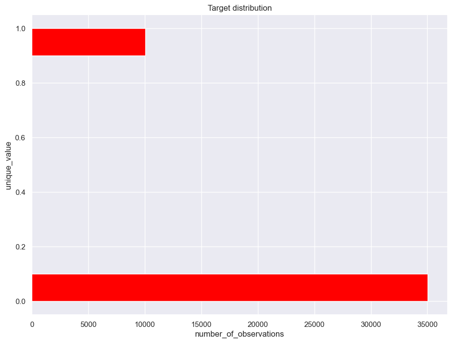
Check the class balance:
ax = data["SeriousDlqin2yrs"].hist(orientation="horizontal", color="red")
ax.set_xlabel("number_of_observations")
ax.set_ylabel("unique_value")
ax.set_title("Target distribution")

print("Distribution of the target:")
data["SeriousDlqin2yrs"].value_counts() / data.shape[0]
Distribution of the target:
SeriousDlqin2yrs
0    0.777511
1    0.222489
Name: count, dtype: float64
Separate the input variable names by excluding the target:
independent_columns_names = [x for x in data if x != "SeriousDlqin2yrs"]
independent_columns_names
['age',
 'NumberOfTime30-59DaysPastDueNotWorse',
 'DebtRatio',
 'NumberOfTimes90DaysLate',
 'NumberOfTime60-89DaysPastDueNotWorse',
 'MonthlyIncome',
 'NumberOfDependents']
Apply the function to replace NaN values:
table = fill_nan(data)
Separate the target variable and input features:
X = table[independent_columns_names]
y = table["SeriousDlqin2yrs"]
Bootstrapping#
Question 2. Make an interval estimate of the average age for the customers who delayed repayment at the 90% confidence level. Use the example from the article as reference, if needed. Also, use np.random.seed(0) as before. What is the resulting interval estimate?
52.59 – 52.86
45.71 – 46.13
45.68 – 46.17
52.56 – 52.88
# You code here (read-only in a JupyterBook, pls run jupyter-notebook to edit)
Logistic regression#
Let’s set up to use logistic regression:
from sklearn.linear_model import LogisticRegression
from sklearn.model_selection import GridSearchCV, StratifiedKFold
Now, we will create a LogisticRegression model and use class_weight='balanced' to make up for our unbalanced classes.
lr = LogisticRegression(random_state=5, class_weight="balanced")
Let’s try to find the best regularization coefficient, which is the coefficient C for logistic regression. Then, we will have an optimal model that is not overfit and is a good predictor of the target variable.
parameters = {"C": (0.0001, 0.001, 0.01, 0.1, 1, 10)}
In order to find the optimal value of C, let’s apply stratified 5-fold validation and look at the ROC AUC against different values of the parameter C. Use the StratifiedKFold function for this:
skf = StratifiedKFold(n_splits=5, shuffle=True, random_state=5)
One of the important metrics of model quality is the Area Under the Curve (AUC). ROC AUC varies from 0 to 1. The closer ROC AUC is to 1, the better the quality of the classification model.
Question 3. Perform a Grid Search with the scoring metric “roc_auc” for the parameter C. Which value of the parameter C is optimal?
0.0001
0.001
0.01
0.1
1
10
# You code here (read-only in a JupyterBook, pls run jupyter-notebook to edit)
Question 4. Can we consider the best model stable? The model is stable if the standard deviation on validation is less than 0.5%. Save the ROC AUC value of the best model; it will be useful for the following tasks.
Yes
No
# You code here (read-only in a JupyterBook, pls run jupyter-notebook to edit)
Feature importance#
Question 5. Feature importance is defined by the absolute value of its corresponding coefficient. First, you need to normalize all of the feature values so that it will be valid to compare them. What is the most important feature for the best logistic regression model?
age
NumberOfTime30-59DaysPastDueNotWorse
DebtRatio
NumberOfTimes90DaysLate
NumberOfTime60-89DaysPastDueNotWorse
MonthlyIncome
NumberOfDependents
# You code here (read-only in a JupyterBook, pls run jupyter-notebook to edit)
Question 6. Calculate how much DebtRatio affects our prediction using the softmax function. What is its value?
0.38
-0.02
0.11
0.24
# You code here (read-only in a JupyterBook, pls run jupyter-notebook to edit)
Question 7. Let’s see how we can interpret the impact of our features. For this, recalculate the logistic regression with absolute values, that is without scaling. Next, modify the customer’s age by adding 20 years, keeping the other features unchanged. How many times will the chance that the customer will not repay their debt increase? You can find an example of the theoretical calculation here.
-0.01
0.70
8.32
0.66
# You code here (read-only in a JupyterBook, pls run jupyter-notebook to edit)
Random Forest#
Import the Random Forest classifier:
from sklearn.ensemble import RandomForestClassifier
Initialize Random Forest with 100 trees and balance target classes:
rf = RandomForestClassifier(
    n_estimators=100, n_jobs=-1, random_state=42, class_weight="balanced"
)
We will search for the best parameters among the following values:
parameters = {
    "max_features": [1, 2, 4],
    "min_samples_leaf": [3, 5, 7, 9],
    "max_depth": [5, 10, 15],
}
Also, we will use the stratified k-fold validation again. You should still have the skf variable.
Question 8. How much higher is the ROC AUC of the best random forest model than that of the best logistic regression on validation? Select the closest answer.
0.04
0.03
0.02
0.01
# You code here (read-only in a JupyterBook, pls run jupyter-notebook to edit)
Question 9. What feature has the weakest impact in the Random Forest model?
age
NumberOfTime30-59DaysPastDueNotWorse
DebtRatio
NumberOfTimes90DaysLate
NumberOfTime60-89DaysPastDueNotWorse
MonthlyIncome
NumberOfDependents
# You code here (read-only in a JupyterBook, pls run jupyter-notebook to edit)
Question 10. What is the most significant advantage of using Logistic Regression versus Random Forest for this problem?
Spent less time for model fitting;
Fewer variables to iterate;
Feature interpretability;
Linear properties of the algorithm.
Bagging#
Import modules and set up the parameters for bagging:
from sklearn.ensemble import BaggingClassifier
from sklearn.model_selection import RandomizedSearchCV, cross_val_score

parameters = {
    "max_features": [2, 3, 4],
    "max_samples": [0.5, 0.7, 0.9],
    "base_estimator__C": [0.0001, 0.001, 0.01, 1, 10, 100],
}
Question 11. Fit a bagging classifier with random_state=42. For the base classifiers, use 100 logistic regressors and use RandomizedSearchCV instead of GridSearchCV. It will take a lot of time to iterate over all 54 variants, so set the maximum number of iterations for RandomizedSearchCV to 20. Don’t forget to set the parameters cv and random_state=1. What is the best ROC AUC you achieve?
80.75%
80.12%
79.62%
76.50%
# You code here (read-only in a JupyterBook, pls run jupyter-notebook to edit)
Question 12. Give an interpretation of the best parameters for bagging. Why are these values of max_features and max_samples the best?
For bagging it’s important to use as few features as possible;
Bagging works better on small samples;
Less correlation between single models;
The higher the number of features, the lower the loss of information.