Topic 8. Vowpal Wabbit: Learning with Gigabytes of Data

mlcourse.ai – Open Machine Learning Course

Author: Yury Kashnitsky. Translated and edited by Serge Oreshkov, and Yuanyuan Pao. This material is subject to the terms and conditions of the Creative Commons CC BY-NC-SA 4.0 license. Free use is permitted for any non-commercial purpose.

This week, we’ll cover two reasons for Vowpal Wabbit’s exceptional training speed, namely, online learning and hashing trick, in both theory and practice. We will try it out with news, movie reviews, and StackOverflow questions.

Article outline

1. Stochastic gradient descent and online learning

   • 1.1. SGD

   • 1.2. Online approach to learning

2. Categorical feature processing

   • 2.1. Label Encoding

   • 2.2. One-Hot Encoding

   • 2.3. Hashing trick

3. Vowpal Wabbit

   • 3.1. News. Binary classification

   • 3.2. News. Multiclass classification

   • 3.3. IMDB movie reviews

   • 3.4. Classifying gigabytes of StackOverflow questions

4. Useful resources

import os
import re

import numpy as np
import pandas as pd
from scipy.sparse import csr_matrix
from sklearn.datasets import fetch_20newsgroups, load_files
from sklearn.linear_model import LogisticRegression
from sklearn.metrics import (accuracy_score, classification_report,
                             confusion_matrix, log_loss, roc_auc_score,
                             roc_curve)
from sklearn.model_selection import train_test_split
from sklearn.preprocessing import LabelEncoder, OneHotEncoder

import matplotlib.pyplot as plt
import seaborn as sns
%config InlineBackend.figure_format = 'retina'

1. Stochastic gradient descent and online learning

1.1. Stochastic gradient descent

Despite the fact that gradient descent is one of the first things learned in machine learning and optimization courses, it is one of its modifications, Stochastic Gradient Descent (SGD), that is hard to top.

Recall that the idea of gradient descent is to minimize some function by making small steps in the direction of the fastest decrease. This method was named due to the following fact from calculus: vector \(\nabla f = (\frac{\partial f}{\partial x_1}, \ldots \frac{\partial f}{\partial x_n})^\text{T}\) of partial derivatives of the function \(f(x) = f(x_1, \ldots x_n)\) points to the direction of the fastest function growth. It means that, by moving in the opposite direction (antigradient), it is possible to decrease the function value with the fastest rate.

Here is a snowboarder (me) in Sheregesh, Russia’s most popular winter resort. (I highly recommended it if you like skiing or snowboarding). In addition to advertising the beautiful landscapes, this picture depicts the idea of gradient descent. If you want to ride as fast as possible, you need to choose the path of steepest descent. Calculating antigradients can be seen as evaluating the slope at various spots.

Example

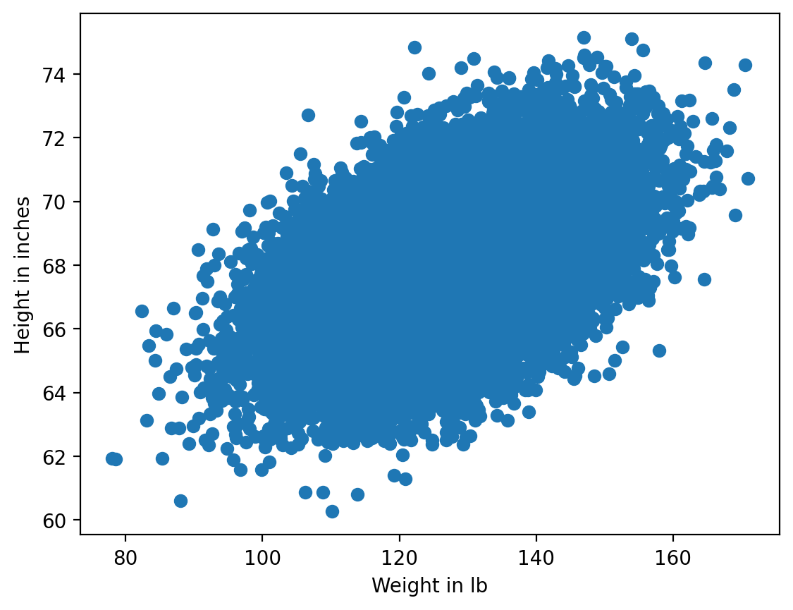
The paired regression problem can be solved with gradient descent. Let us predict one variable using another: height with weight. Assume that these variables are linearly dependent. We will use the SOCR dataset.

# for Jupyter-book, we copy data from GitHub, locally, to save Internet traffic,
# you can specify the data/ folder from the root of your cloned
# https://github.com/Yorko/mlcourse.ai repo, to save Internet traffic
DATA_PATH = "https://raw.githubusercontent.com/Yorko/mlcourse.ai/main/data/"

PATH_TO_WRITE_DATA = "../../../data/tmp/"
data_demo = pd.read_csv(os.path.join(DATA_PATH, "weights_heights.csv"))

plt.scatter(data_demo["Weight"], data_demo["Height"])
plt.xlabel("Weight in lb")
plt.ylabel("Height in inches");

Here we have a vector \(x\) of dimension \(\ell\) (weight of every person i.e. training sample) and \(y\), a vector containing the height of every person in the dataset.

The task is the following: find weights \(w_0\) and \(w_1\) such that predicting height as \(y_i = w_0 + w_1 x_i\) (where \(y_i\) is \(i\)-th height value, \(x_i\) is \(i\)-th weight value) minimizes the squared error (as well as mean squared error since \(\frac{1}{\ell}\) doesn’t make any difference ):

\[ SE(w_0, w_1) = \frac{1}{2}\sum_{i=1}^\ell(y_i - (w_0 + w_1x_{i}))^2 \rightarrow min_{w_0,w_1} \]

We will use gradient descent, utilizing the partial derivatives of \(SE(w_0, w_1)\) over weights \(w_0\) and \(w_1\). An iterative training procedure is then defined by simple update formulas (we change model weights in small steps, proportional to a small constant \(\eta\), towards the antigradient of the function \(SE(w_0, w_1)\)):

\[\begin{split} \begin{array}{rcl} w_0^{(t+1)} = w_0^{(t)} -\eta \frac{\partial SE}{\partial w_0} |_{t} \\ w_1^{(t+1)} = w_1^{(t)} -\eta \frac{\partial SE}{\partial w_1} |_{t} \end{array} \end{split}\]

Computing the partial derivatives, we get the following:

\[\begin{split} \begin{array}{rcl} w_0^{(t+1)} = w_0^{(t)} + \eta \sum_{i=1}^{\ell}(y_i - w_0^{(t)} - w_1^{(t)}x_i) \\ w_1^{(t+1)} = w_1^{(t)} + \eta \sum_{i=1}^{\ell}(y_i - w_0^{(t)} - w_1^{(t)}x_i)x_i \end{array} \end{split}\]

This math works quite well as long as the amount of data is not large (we will not discuss issues with local minima, saddle points, choosing the learning rate, moments and other stuff –- these topics are covered very thoroughly in the Numeric Computation chapter in “Deep Learning”). There is an issue with batch gradient descent – the gradient evaluation requires the summation of a number of values for every object from the training set. In other words, the algorithm requires a lot of iterations, and every iteration recomputes weights with formula which contains a sum \(\sum_{i=1}^\ell\) over the whole training set. What happens when we have billions of training samples?

Hence the motivation for stochastic gradient descent! Simply put, we throw away the summation sign and update the weights only over single training samples (or a small number of them). In our case, we have the following:

\[\begin{split} \begin{array}{rcl} w_0^{(t+1)} = w_0^{(t)} + \eta (y_i - w_0^{(t)} - w_1^{(t)}x_i) \\ w_1^{(t+1)} = w_1^{(t)} + \eta (y_i - w_0^{(t)} - w_1^{(t)}x_i)x_i \end{array} \end{split}\]

With this approach, there is no guarantee that we will move in best possible direction at every iteration. Therefore, we may need many more iterations, but we get much faster weight updates.

Andrew Ng has a good illustration of this in his machine learning course. Let’s take a look.

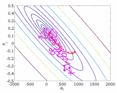
These are the contour plots for some function, and we want to find the global minimum of this function. The red curve shows weight changes (in this picture, \(\theta_0\) and \(\theta_1\) correspond to our \(w_0\) and \(w_1\)). According to the properties of a gradient, the direction of change at every point is orthogonal to contour plots. With stochastic gradient descent, weights are changing in a less predictable manner, and it even may seem that some steps are wrong by leading away from minima; however, both procedures converge to the same solution.

1.2. Online approach to learning

Stochastic gradient descent gives us practical guidance for training both classifiers and regressors with large amounts of data up to hundreds of GBs (depending on computational resources).

Considering the case of paired regression, we can store the training data set \((X,y)\) in HDD without loading it into RAM (where it simply won’t fit), read objects one by one, and update the weights of our model:

\[\begin{split} \begin{array}{rcl} w_0^{(t+1)} = w_0^{(t)} + \eta (y_i - w_0^{(t)} - w_1^{(t)}x_i) \\ w_1^{(t+1)} = w_1^{(t)} + \eta (y_i - w_0^{(t)} - w_1^{(t)}x_i)x_i \end{array} \end{split}\]

After working through the whole training dataset, our loss function (for example, quadratic squared root error in regression or logistic loss in classification) will decrease, but it usually takes dozens of passes over the training set to make the loss small enough.

This approach to learning is called online learning, and this name emerged even before machine learning MOOC-s turned mainstream.

We did not discuss many specifics about SGD here. If you want dive into theory, I highly recommend “Convex Optimization” by Stephen Boyd. Now, we will introduce the Vowpal Wabbit library, which is good for training simple models with huge data sets thanks to stochastic optimization and another trick, feature hashing.

In scikit-learn, classifiers and regressors trained with SGD are named SGDClassifier and SGDRegressor in sklearn.linear_model. These are nice implementations of SGD, but we’ll focus on VW since it is more performant than sklearn’s SGD models in many aspects.

2. Categorical feature processing

2.1. Label Encoding

Many classification and regression algorithms operate in Euclidean or metric space, implying that data is represented with vectors of real numbers. However, in real data, we often have categorical features with discrete values such as yes/no or January/February/…/December. We will see how to process this kind of data, particularly with linear models, and how to deal with many categorical features even when they have many unique values.

Let’s explore the UCI bank marketing dataset where most of features are categorical.

df = pd.read_csv(os.path.join(DATA_PATH, "bank_train.csv"))
labels = pd.read_csv(
    os.path.join(DATA_PATH, "bank_train_target.csv"), header=None
)

df.head()

	age	job	marital	education	default	housing	loan	contact	month	day_of_week	duration	campaign	pdays	previous	poutcome	emp.var.rate	cons.price.idx	cons.conf.idx	euribor3m	nr.employed
0	26	student	single	high.school	no	no	no	telephone	jun	mon	901	1	999	0	nonexistent	1.4	94.465	-41.8	4.961	5228.1
1	46	admin.	married	university.degree	no	yes	no	cellular	aug	tue	208	2	999	0	nonexistent	1.4	93.444	-36.1	4.963	5228.1
2	49	blue-collar	married	basic.4y	unknown	yes	yes	telephone	jun	tue	131	5	999	0	nonexistent	1.4	94.465	-41.8	4.864	5228.1
3	31	technician	married	university.degree	no	no	no	cellular	jul	tue	404	1	999	0	nonexistent	-2.9	92.469	-33.6	1.044	5076.2
4	42	housemaid	married	university.degree	no	yes	no	telephone	nov	mon	85	1	999	0	nonexistent	-0.1	93.200	-42.0	4.191	5195.8

We can see that most of features are not represented by numbers. This poses a problem because we cannot use most machine learning methods (at least those implemented in scikit-learn) out-of-the-box.

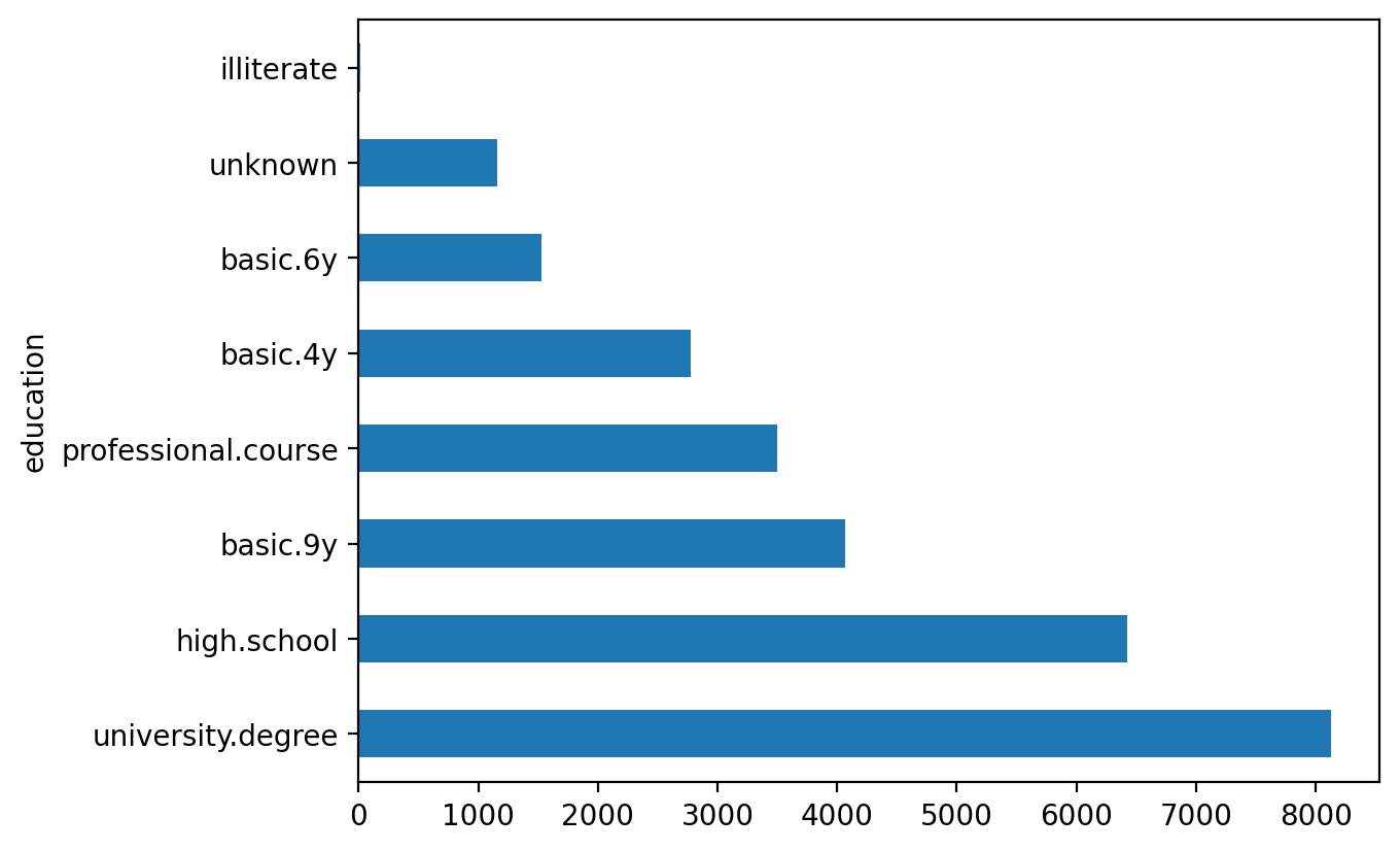
Let’s dive into the “education” feature.

df["education"].value_counts().plot.barh();

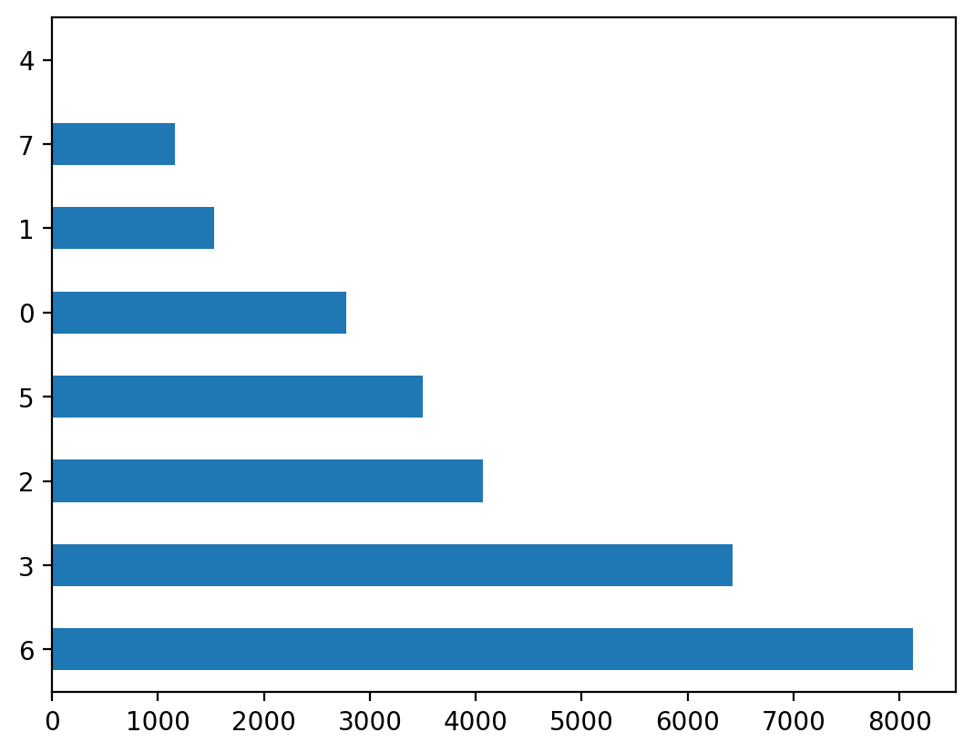
The most straightforward solution is to map each value of this feature into a unique number. For example, we can map university.degree to 0, basic.9y to 1, and so on. You can use sklearn.preprocessing.LabelEncoder to perform this mapping.

label_encoder = LabelEncoder()

The fit method of this class finds all unique values and builds the actual mapping between categories and numbers, and the transform method converts the categories into numbers. After fit is executed, label_encoder will have the classes_ attribute with all unique values of the feature. Let us count them to make sure the transformation was correct.

mapped_education = pd.Series(label_encoder.fit_transform(df["education"]))
mapped_education.value_counts().plot.barh()
print(dict(enumerate(label_encoder.classes_)))

{0: 'basic.4y', 1: 'basic.6y', 2: 'basic.9y', 3: 'high.school', 4: 'illiterate', 5: 'professional.course', 6: 'university.degree', 7: 'unknown'}

df["education"] = mapped_education
df.head()

	age	job	marital	education	default	housing	loan	contact	month	day_of_week	duration	campaign	pdays	previous	poutcome	emp.var.rate	cons.price.idx	cons.conf.idx	euribor3m	nr.employed
0	26	student	single	3	no	no	no	telephone	jun	mon	901	1	999	0	nonexistent	1.4	94.465	-41.8	4.961	5228.1
1	46	admin.	married	6	no	yes	no	cellular	aug	tue	208	2	999	0	nonexistent	1.4	93.444	-36.1	4.963	5228.1
2	49	blue-collar	married	0	unknown	yes	yes	telephone	jun	tue	131	5	999	0	nonexistent	1.4	94.465	-41.8	4.864	5228.1
3	31	technician	married	6	no	no	no	cellular	jul	tue	404	1	999	0	nonexistent	-2.9	92.469	-33.6	1.044	5076.2
4	42	housemaid	married	6	no	yes	no	telephone	nov	mon	85	1	999	0	nonexistent	-0.1	93.200	-42.0	4.191	5195.8

Let’s apply the transformation to other columns of type object.

categorical_columns = df.columns[df.dtypes == "object"].union(["education"])
for column in categorical_columns:
    df[column] = label_encoder.fit_transform(df[column])
df.head()

	age	job	marital	education	default	housing	loan	contact	month	day_of_week	duration	campaign	pdays	previous	poutcome	emp.var.rate	cons.price.idx	cons.conf.idx	euribor3m	nr.employed
0	26	8	2	3	0	0	0	1	4	1	901	1	999	0	1	1.4	94.465	-41.8	4.961	5228.1
1	46	0	1	6	0	2	0	0	1	3	208	2	999	0	1	1.4	93.444	-36.1	4.963	5228.1
2	49	1	1	0	1	2	2	1	4	3	131	5	999	0	1	1.4	94.465	-41.8	4.864	5228.1
3	31	9	1	6	0	0	0	0	3	3	404	1	999	0	1	-2.9	92.469	-33.6	1.044	5076.2
4	42	3	1	6	0	2	0	1	7	1	85	1	999	0	1	-0.1	93.200	-42.0	4.191	5195.8

The main issue with this approach is that we have now introduced some relative ordering where it might not exist.

For example, we implicitly introduced algebra over the values of the job feature where we can now substract the job of client #2 from the job of client #1 :

df.loc[1].job - df.loc[2].job

np.float64(-1.0)

Does this operation make any sense? Not really. Let’s try to train logistic regression with this feature transformation.

def logistic_regression_accuracy_on(dataframe, labels):
    features = dataframe
    train_features, test_features, train_labels, test_labels = train_test_split(
        features, labels
    )

    logit = LogisticRegression()
    logit.fit(train_features, train_labels)
    return classification_report(test_labels, logit.predict(test_features))


print(logistic_regression_accuracy_on(df[categorical_columns], labels))

              precision    recall  f1-score   support

           0       0.89      1.00      0.94      6130
           1       1.00      0.00      0.00       769

    accuracy                           0.89      6899
   macro avg       0.94      0.50      0.47      6899
weighted avg       0.90      0.89      0.84      6899

/Users/kashnitsky/Library/Caches/pypoetry/virtualenvs/mlcourse-ai-czBTtoES-py3.12/lib/python3.12/site-packages/sklearn/utils/validation.py:1310: DataConversionWarning: A column-vector y was passed when a 1d array was expected. Please change the shape of y to (n_samples, ), for example using ravel().
  y = column_or_1d(y, warn=True)

We can see that logistic regression never predicts class 1. In order to use linear models with categorical features, we will use a different approach: One-Hot Encoding.

2.2. One-Hot Encoding

Suppose that some feature can have one of 10 unique values. One-hot encoding creates 10 new features corresponding to these unique values, all of them except one are zeros.

one_hot_example = pd.DataFrame([{i: 0 for i in range(10)}])
one_hot_example.loc[0, 6] = 1
one_hot_example

	0	1	2	3	4	5	6	7	8	9
0	0	0	0	0	0	0	1	0	0	0

This idea is implemented in the OneHotEncoder class from sklearn.preprocessing. By default OneHotEncoder transforms data into a sparse matrix to save memory space because most of the values are zeroes and because we do not want to take up more RAM. However, in this particular example, we do not encounter such problems, so we are going to use a “dense” matrix representation.

onehot_encoder = OneHotEncoder(sparse_output=False)

encoded_categorical_columns = pd.DataFrame(
    onehot_encoder.fit_transform(df[categorical_columns])
)
encoded_categorical_columns.head()

	0	1	2	3	4	5	6	7	8	9	...	43	44	45	46	47	48	49	50	51	52
0	0.0	1.0	0.0	1.0	0.0	0.0	0.0	1.0	0.0	0.0	...	0.0	1.0	0.0	0.0	0.0	0.0	0.0	0.0	1.0	0.0
1	1.0	0.0	0.0	0.0	0.0	1.0	0.0	1.0	0.0	0.0	...	0.0	0.0	0.0	0.0	0.0	0.0	0.0	0.0	1.0	0.0
2	0.0	1.0	0.0	0.0	0.0	1.0	0.0	0.0	1.0	0.0	...	0.0	1.0	0.0	0.0	0.0	0.0	0.0	0.0	1.0	0.0
3	1.0	0.0	0.0	0.0	0.0	1.0	0.0	1.0	0.0	0.0	...	1.0	0.0	0.0	0.0	0.0	0.0	0.0	0.0	1.0	0.0
4	0.0	1.0	0.0	1.0	0.0	0.0	0.0	1.0	0.0	0.0	...	0.0	0.0	0.0	0.0	1.0	0.0	0.0	0.0	1.0	0.0

5 rows × 53 columns

We have 53 columns that correspond to the number of unique values of categorical features in our data set. When transformed with One-Hot Encoding, this data can be used with linear models:

print(logistic_regression_accuracy_on(encoded_categorical_columns, labels))

              precision    recall  f1-score   support

           0       0.90      0.99      0.94      6118
           1       0.63      0.18      0.28       781

    accuracy                           0.90      6899
   macro avg       0.77      0.58      0.61      6899
weighted avg       0.87      0.90      0.87      6899

/Users/kashnitsky/Library/Caches/pypoetry/virtualenvs/mlcourse-ai-czBTtoES-py3.12/lib/python3.12/site-packages/sklearn/utils/validation.py:1310: DataConversionWarning: A column-vector y was passed when a 1d array was expected. Please change the shape of y to (n_samples, ), for example using ravel().
  y = column_or_1d(y, warn=True)

2.3. Hashing trick

Real data can be volatile, meaning we cannot guarantee that new values of categorical features will not occur. This issue hampers using a trained model on new data. Besides that, LabelEncoder requires preliminary analysis of the whole dataset and storage of constructed mappings in memory, which makes it difficult to work with large datasets.

There is a simple approach to vectorization of categorical data based on hashing and is known as, not-so-surprisingly, the hashing trick.

Hash functions can help us find unique codes for different feature values, for example:

for s in ("university.degree", "high.school", "illiterate"):
    print(s, "->", hash(s))

university.degree -> -8301455830773922005
high.school -> -7087776842577270240
illiterate -> -5724181697257202701

We will not use negative values or values of high magnitude, so we restrict the range of values for the hash function:

hash_space = 25
for s in ("university.degree", "high.school", "illiterate"):
    print(s, "->", hash(s) % hash_space)

university.degree -> 20
high.school -> 10
illiterate -> 24

Imagine that our data set contains a single (i.e. not married) student, who received a call on Monday. His feature vectors will be created similarly as in the case of One-Hot Encoding but in the space with fixed range for all features:

hashing_example = pd.DataFrame([{i: 0.0 for i in range(hash_space)}])
for s in ("job=student", "marital=single", "day_of_week=mon"):
    print(s, "->", hash(s) % hash_space)
    hashing_example.loc[0, hash(s) % hash_space] = 1
hashing_example

job=student -> 4
marital=single -> 24
day_of_week=mon -> 16

	0	1	2	3	4	5	6	7	8	9	...	15	16	17	18	19	20	21	22	23	24
0	0.0	0.0	0.0	0.0	1.0	0.0	0.0	0.0	0.0	0.0	...	0.0	1.0	0.0	0.0	0.0	0.0	0.0	0.0	0.0	1.0

1 rows × 25 columns

We want to point out that we hash not only feature values but also pairs of feature name + feature value. It is important to do this so that we can distinguish the same values of different features.

assert hash("no") == hash("no")
assert hash("housing=no") != hash("loan=no")

Is it possible to have a collision when using hash codes? Sure, it is possible, but it is a rare case with large enough hashing spaces. Even if collision occurs, regression or classification metrics will not suffer much. In this case, hash collisions work as a form of regularization.

You may be saying “WTF?”; hashing seems counterintuitive. This is true, but these heuristics sometimes are, in fact, the only plausible approach to work with categorical data (what else can you do if you have 30M features?). Moreover, this technique has proven to just work. As you work more with data, you may see this for yourself.

A good analysis of hash collisions, their dependency on feature space and hashing space dimensions and affecting classification/regression performance is done in this article by Booking.com.

3. Vowpal Wabbit

Vowpal Wabbit (VW) is one of the most widespread machine learning libraries used in industry. It is prominent for its training speed and support of many training modes, especially for online learning with big and high-dimensional data. This is one of the major merits of the library. Also, with the hashing trick implemented, Vowpal Wabbit is a perfect choice for working with text data.

Shell is the main interface for VW.

#!vw --help | head

Vowpal Wabbit reads data from files or from standard input stream (stdin) with the following format:

[Label] [Importance] [Tag]|Namespace Features |Namespace Features ... |Namespace Features

Namespace=String[:Value]

Features=(String[:Value] )*

here [] denotes non-mandatory elements, and (…)* means multiple inputs allowed.

• Label is a number. In the case of classification, it is usually 1 and -1; for regression, it is a real float value

• Importance is a number. It denotes the sample weight during training. Setting this helps when working with imbalanced data.

• Tag is a string without spaces. It is the “name” of the sample that VW saves upon prediction. In order to separate Tag from Importance, it is better to start Tag with the ‘ character.

• Namespace is for creating different feature spaces.

• Features are object features inside a given Namespace. Features have weight 1.0 by default, but it can be changed, for example feature:0.1.

The following string matches the VW format:

1 1.0 |Subject WHAT car is this |Organization University of Maryland:0.5 College Park

Let’s check the format by running VW with this training sample:

! echo '1 1.0 |Subject WHAT car is this |Organization University of Maryland:0.5 College Park' | vw

/bin/bash: line 1: 41549 Done                    echo '1 1.0 |Subject WHAT car is this |Organization University of Maryland:0.5 College Park'
     41550 Killed: 9               | vw

VW is a wonderful tool for working with text data. We’ll illustrate it with the 20newsgroups dataset, which contains letters from 20 different newsletters.

3.1. News. Binary classification.

# load data with sklearn's function
newsgroups = fetch_20newsgroups(data_home=PATH_TO_WRITE_DATA)

newsgroups["target_names"]

['alt.atheism',
 'comp.graphics',
 'comp.os.ms-windows.misc',
 'comp.sys.ibm.pc.hardware',
 'comp.sys.mac.hardware',
 'comp.windows.x',
 'misc.forsale',
 'rec.autos',
 'rec.motorcycles',
 'rec.sport.baseball',
 'rec.sport.hockey',
 'sci.crypt',
 'sci.electronics',
 'sci.med',
 'sci.space',
 'soc.religion.christian',
 'talk.politics.guns',
 'talk.politics.mideast',
 'talk.politics.misc',
 'talk.religion.misc']

Lets look at the first document in this collection:

text = newsgroups["data"][0]
target = newsgroups["target_names"][newsgroups["target"][0]]

print("-----")
print(target)
print("-----")
print(text.strip())
print("----")

-----
rec.autos
-----
From: lerxst@wam.umd.edu (where's my thing)
Subject: WHAT car is this!?
Nntp-Posting-Host: rac3.wam.umd.edu
Organization: University of Maryland, College Park
Lines: 15

 I was wondering if anyone out there could enlighten me on this car I saw
the other day. It was a 2-door sports car, looked to be from the late 60s/
early 70s. It was called a Bricklin. The doors were really small. In addition,
the front bumper was separate from the rest of the body. This is 
all I know. If anyone can tellme a model name, engine specs, years
of production, where this car is made, history, or whatever info you
have on this funky looking car, please e-mail.

Thanks,
- IL
   ---- brought to you by your neighborhood Lerxst ----
----

Now we convert the data into something Vowpal Wabbit can understand. We will throw away words shorter than 3 symbols. Here, we will skip some important NLP stages such as stemming and lemmatization; however, we will later see that VW solves the problem even without these steps.

def to_vw_format(document, label=None):
    return (
        str(label or "")
        + " |text "
        + " ".join(re.findall("\w{3,}", document.lower()))
        + "\n"
    )


to_vw_format(text, 1 if target == "rec.autos" else -1)

<>:5: SyntaxWarning: invalid escape sequence '\w'
<>:5: SyntaxWarning: invalid escape sequence '\w'
/var/folders/n0/1qj4_6k97ms4rnr_bsfq6j40018_cq/T/ipykernel_41494/1433298466.py:5: SyntaxWarning: invalid escape sequence '\w'
  + " ".join(re.findall("\w{3,}", document.lower()))

'1 |text from lerxst wam umd edu where thing subject what car this nntp posting host rac3 wam umd edu organization university maryland college park lines was wondering anyone out there could enlighten this car saw the other day was door sports car looked from the late 60s early 70s was called bricklin the doors were really small addition the front bumper was separate from the rest the body this all know anyone can tellme model name engine specs years production where this car made history whatever info you have this funky looking car please mail thanks brought you your neighborhood lerxst\n'

We split the dataset into train and test and write these into separate files. We will consider a document as positive if it corresponds to rec.autos. Thus, we are constructing a model which distinguishes articles about cars from other topics:

all_documents = newsgroups["data"]
all_targets = [
    1 if newsgroups["target_names"][target] == "rec.autos" else -1
    for target in newsgroups["target"]
]

train_documents, test_documents, train_labels, test_labels = train_test_split(
    all_documents, all_targets, random_state=7
)

with open(os.path.join(PATH_TO_WRITE_DATA, "20news_train.vw"), "w") as vw_train_data:
    for text, target in zip(train_documents, train_labels):
        vw_train_data.write(to_vw_format(text, target))
with open(os.path.join(PATH_TO_WRITE_DATA, "20news_test.vw"), "w") as vw_test_data:
    for text in test_documents:
        vw_test_data.write(to_vw_format(text))

Now, we pass the created training file to Vowpal Wabbit. We solve the classification problem with a hinge loss function (linear SVM). The trained model will be saved in the 20news_model.vw file:

#!vw -d $PATH_TO_WRITE_DATA/20news_train.vw \
# --loss_function hinge -f $PATH_TO_WRITE_DATA/20news_model.vw

VW prints a lot of interesting info while training (one can suppress it with the --quiet parameter). You can see documentation of the diagnostic output. Note how average loss drops while training. For loss computation, VW uses samples it has never seen before, so this measure is usually accurate. Now, we apply our trained model to the test set, saving predictions into a file with the -p flag:

#!vw -i $PATH_TO_WRITE_DATA/20news_model.vw -t -d $PATH_TO_WRITE_DATA/20news_test.vw \
# -p $PATH_TO_WRITE_DATA/20news_test_predictions.txt

Now we load our predictions, compute AUC, and plot the ROC curve:

with open(os.path.join(PATH_TO_WRITE_DATA, "20news_test_predictions.txt")) as pred_file:
    test_prediction = [float(label) for label in pred_file.readlines()]

auc = roc_auc_score(test_labels, test_prediction)
roc_curve = roc_curve(test_labels, test_prediction)


plt.plot(roc_curve[0], roc_curve[1])
plt.plot([0, 1], [0, 1])
plt.xlabel("FPR")
plt.ylabel("TPR")
plt.title("test AUC = %f" % (auc))
plt.axis([-0.05, 1.05, -0.05, 1.05]);

---------------------------------------------------------------------------
FileNotFoundError                         Traceback (most recent call last)
Cell In[29], line 1
----> 1 with open(os.path.join(PATH_TO_WRITE_DATA, "20news_test_predictions.txt")) as pred_file:
      2     test_prediction = [float(label) for label in pred_file.readlines()]
      4 auc = roc_auc_score(test_labels, test_prediction)

File ~/Library/Caches/pypoetry/virtualenvs/mlcourse-ai-czBTtoES-py3.12/lib/python3.12/site-packages/IPython/core/interactiveshell.py:324, in _modified_open(file, *args, **kwargs)
    317 if file in {0, 1, 2}:
    318     raise ValueError(
    319         f"IPython won't let you open fd={file} by default "
    320         "as it is likely to crash IPython. If you know what you are doing, "
    321         "you can use builtins' open."
    322     )
--> 324 return io_open(file, *args, **kwargs)

FileNotFoundError: [Errno 2] No such file or directory: '../../../data/tmp/20news_test_predictions.txt'

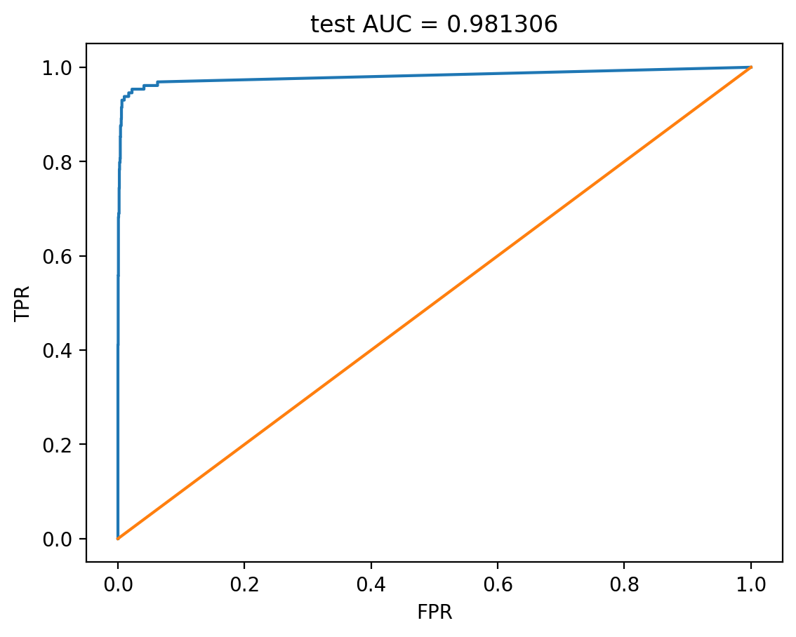
The AUC value we get shows that we have achieved high classification quality.

3.2. News. Multiclass classification

We will use the same news dataset, but, this time, we will solve a multiclass classification problem. Vowpal Wabbit is a little picky – it wants labels starting from 1 till K, where K – is the number of classes in the classification task (20 in our case). So we will use LabelEncoder and add 1 afterwards (recall that LabelEncoder maps labels into range from 0 to K-1).

all_documents = newsgroups["data"]
topic_encoder = LabelEncoder()
all_targets_mult = topic_encoder.fit_transform(newsgroups["target"]) + 1

The data is the same, but we have changed the labels, train_labels_mult and test_labels_mult, into label vectors from 1 to 20.

train_documents, test_documents, train_labels_mult, test_labels_mult = train_test_split(
    all_documents, all_targets_mult, random_state=7
)

with open(os.path.join(PATH_TO_WRITE_DATA, "20news_train_mult.vw"), "w") as vw_train_data:
    for text, target in zip(train_documents, train_labels_mult):
        vw_train_data.write(to_vw_format(text, target))
with open(os.path.join(PATH_TO_WRITE_DATA, "20news_test_mult.vw"), "w") as vw_test_data:
    for text in test_documents:
        vw_test_data.write(to_vw_format(text))

We train Vowpal Wabbit in multiclass classification mode, passing the oaa parameter(“one against all”) with the number of classes. Also, let’s see what parameters our model quality is dependent on (more info can be found in the official Vowpal Wabbit tutorial):

• learning rate (-l, 0.5 default) – rate of weight change on every step

• learning rate decay (–power_t, 0.5 default) – it is proven in practice, that, if the learning rate drops with the number of steps in stochastic gradient descent, we approach the minimum loss better

• loss function (–loss_function) – the entire training algorithm depends on it. See docs for loss functions

• Regularization (-l1) – note that VW calculates regularization for every object. That is why we usually set regularization values to about \(10^{-20}.\)

Additionally, we can try automatic Vowpal Wabbit parameter tuning with Hyperopt.

#!vw --oaa 20 $PATH_TO_WRITE_DATA/20news_train_mult.vw -f $PATH_TO_WRITE_DATA/ \
#20news_model_mult.vw --loss_function=hinge

#%%time
#!vw -i $PATH_TO_WRITE_DATA/20news_model_mult.vw -t -d $PATH_TO_WRITE_DATA/20news_test_mult.vw \
#-p $PATH_TO_WRITE_DATA/20news_test_predictions_mult.txt

with open(
    os.path.join(PATH_TO_WRITE_DATA, "20news_test_predictions_mult.txt")
) as pred_file:
    test_prediction_mult = [float(label) for label in pred_file.readlines()]

accuracy_score(test_labels_mult, test_prediction_mult)

Here is how often the model misclassifies atheism with other topics:

M = confusion_matrix(test_labels_mult, test_prediction_mult)
for i in np.where(M[0, :] > 0)[0][1:]:
    print(newsgroups["target_names"][i], M[0, i])

3.3. IMDB movie reviews

In this part we will do binary classification of IMDB (International Movie DataBase) movie reviews. We will see how fast Vowpal Wabbit performs.

Using the load_files function from sklearn.datasets, we load the movie reviews datasets. It’s the same dataset we used in topic04 part4 notebook.

import tarfile
# Download the dataset if not already in place
from io import BytesIO

import requests

url = "http://ai.stanford.edu/~amaas/data/sentiment/aclImdb_v1.tar.gz"


def load_imdb_dataset(extract_path=PATH_TO_WRITE_DATA, overwrite=False):
    # check if existed already
    if (
        os.path.isfile(os.path.join(extract_path, "aclImdb", "README"))
        and not overwrite
    ):
        print("IMDB dataset is already in place.")
        return

    print("Downloading the dataset from:  ", url)
    response = requests.get(url)

    tar = tarfile.open(mode="r:gz", fileobj=BytesIO(response.content))

    data = tar.extractall(extract_path)


load_imdb_dataset()

Read train data, separate labels.

PATH_TO_IMDB = PATH_TO_WRITE_DATA + "aclImdb"

reviews_train = load_files(
    os.path.join(PATH_TO_IMDB, "train"), categories=["pos", "neg"]
)

text_train, y_train = reviews_train.data, reviews_train.target

print("Number of documents in training data: %d" % len(text_train))
print(np.bincount(y_train))

Do the same for the test set.

reviews_test = load_files(os.path.join(PATH_TO_IMDB, "test"), categories=["pos", "neg"])
text_test, y_test = reviews_test.data, reviews_test.target

print("Number of documents in test data: %d" % len(text_test))
print(np.bincount(y_test))

Take a look at examples of reviews and their corresponding labels.

text_train[0]

y_train[0]  # good review

text_train[1]

y_train[1]  # bad review

to_vw_format(str(text_train[1]), 1 if y_train[0] == 1 else -1)

Now, we prepare training (movie_reviews_train.vw), validation (movie_reviews_valid.vw), and test (movie_reviews_test.vw) sets for Vowpal Wabbit. We will use 70% for training, 30% for the hold-out set.

train_share = int(0.7 * len(text_train))
train, valid = text_train[:train_share], text_train[train_share:]
train_labels, valid_labels = y_train[:train_share], y_train[train_share:]

len(train_labels), len(valid_labels)

with open(
    os.path.join(PATH_TO_WRITE_DATA, "movie_reviews_train.vw"), "w"
) as vw_train_data:
    for text, target in zip(train, train_labels):
        vw_train_data.write(to_vw_format(str(text), 1 if target == 1 else -1))
with open(
    os.path.join(PATH_TO_WRITE_DATA, "movie_reviews_valid.vw"), "w"
) as vw_train_data:
    for text, target in zip(valid, valid_labels):
        vw_train_data.write(to_vw_format(str(text), 1 if target == 1 else -1))
with open(os.path.join(PATH_TO_WRITE_DATA, "movie_reviews_test.vw"), "w") as vw_test_data:
    for text in text_test:
        vw_test_data.write(to_vw_format(str(text)))

!head -2 $PATH_TO_WRITE_DATA/movie_reviews_train.vw

!head -2 $PATH_TO_WRITE_DATA/movie_reviews_valid.vw

!head -2 $PATH_TO_WRITE_DATA/movie_reviews_test.vw

Now we launch Vowpal Wabbit with the following arguments:

• -d, path to training set (corresponding .vw file)

• --loss_function – hinge (feel free to experiment here)

• -f – path to the output file (which can also be in the .vw format)

#!vw -d $PATH_TO_WRITE_DATA/movie_reviews_train.vw --loss_function hinge \
#-f $PATH_TO_WRITE_DATA/movie_reviews_model.vw --quiet

Next, make the hold-out prediction with the following VW arguments:

• -i –path to the trained model (.vw file)

• -d – path to the hold-out set (.vw file)

• -p – path to a txt-file where the predictions will be stored

• -t - tells VW to ignore labels

#!vw -i $PATH_TO_WRITE_DATA/movie_reviews_model.vw -t \
#-d $PATH_TO_WRITE_DATA/movie_reviews_valid.vw -p $PATH_TO_WRITE_DATA/movie_valid_pred.txt --quiet

Read the predictions from the text file and estimate the accuracy and ROC AUC. Note that VW prints probability estimates of the +1 class. These estimates are distributed from -1 to 1, so we can convert these into binary answers, assuming that positive values belong to class 1.

with open(os.path.join(PATH_TO_WRITE_DATA, "movie_valid_pred.txt")) as pred_file:
    valid_prediction = [float(label) for label in pred_file.readlines()]
print(
    "Accuracy: {}".format(
        round(
            accuracy_score(
                valid_labels, [int(pred_prob > 0) for pred_prob in valid_prediction]
            ),
            3,
        )
    )
)
print("AUC: {}".format(round(roc_auc_score(valid_labels, valid_prediction), 3)))

Again, do the same for the test set.

#!vw -i $PATH_TO_WRITE_DATA/movie_reviews_model.vw -t \
#-d $PATH_TO_WRITE_DATA/movie_reviews_test.vw \
#-p $PATH_TO_WRITE_DATA/movie_test_pred.txt --quiet

with open(os.path.join(PATH_TO_WRITE_DATA, "movie_test_pred.txt")) as pred_file:
    test_prediction = [float(label) for label in pred_file.readlines()]
print(
    "Accuracy: {}".format(
        round(
            accuracy_score(
                y_test, [int(pred_prob > 0) for pred_prob in test_prediction]
            ),
            3,
        )
    )
)
print("AUC: {}".format(round(roc_auc_score(y_test, test_prediction), 3)))

Let’s try to achieve a higher accuracy by incorporating bigrams.

#!vw -d $PATH_TO_WRITE_DATA/movie_reviews_train.vw \
# --loss_function hinge --ngram 2 -f $PATH_TO_WRITE_DATA/movie_reviews_model2.vw --quiet

#!vw -i$PATH_TO_WRITE_DATA/movie_reviews_model2.vw -t -d $PATH_TO_WRITE_DATA/movie_reviews_valid.vw \
#-p $PATH_TO_WRITE_DATA/movie_valid_pred2.txt --quiet

with open(os.path.join(PATH_TO_WRITE_DATA, "movie_valid_pred2.txt")) as pred_file:
    valid_prediction = [float(label) for label in pred_file.readlines()]
print(
    "Accuracy: {}".format(
        round(
            accuracy_score(
                valid_labels, [int(pred_prob > 0) for pred_prob in valid_prediction]
            ),
            3,
        )
    )
)
print("AUC: {}".format(round(roc_auc_score(valid_labels, valid_prediction), 3)))

#!vw -i $PATH_TO_WRITE_DATA/movie_reviews_model2.vw -t -d $PATH_TO_WRITE_DATA/movie_reviews_test.vw \
#-p $PATH_TO_WRITE_DATA/movie_test_pred2.txt --quiet

with open(os.path.join(PATH_TO_WRITE_DATA, "movie_test_pred2.txt")) as pred_file:
    test_prediction2 = [float(label) for label in pred_file.readlines()]
print(
    "Accuracy: {}".format(
        round(
            accuracy_score(
                y_test, [int(pred_prob > 0) for pred_prob in test_prediction2]
            ),
            3,
        )
    )
)
print("AUC: {}".format(round(roc_auc_score(y_test, test_prediction2), 3)))

Adding bigrams really helped to improve our model!

3.4. Classifying gigabytes of StackOverflow questions

This section has been moved to Kaggle, please explore this Notebook.

4. Useful resources

• The same notebook as am interactive web-based Kaggle Kernel

• “Training while reading” - an example of the Python wrapper usage

• Main course site, course repo, and YouTube channel

• Course materials as a Kaggle Dataset

• Official VW documentation on Github

• “Awesome Vowpal Wabbit” Wiki

• Don’t be tricked by the Hashing Trick - analysis of hash collisions, their dependency on feature space and hashing space dimensions and affecting classification/regression performance

• “Numeric Computation” Chapter of the Deep Learning book

• “Convex Optimization” by Stephen Boyd

• “Command-line Tools can be 235x Faster than your Hadoop Cluster” post

• Benchmarking various ML algorithms on Criteo 1TB dataset on GitHub

• VW on FastML.com