Assignment #7 (demo). Unsupervised learning. Solution#

Authors: Olga Daykhovskaya, Yury Kashnitsky. This material is subject to the terms and conditions of the Creative Commons CC BY-NC-SA 4.0 license. Free use is permitted for any non-commercial purpose.
Same assignment as a Kaggle Notebook + solution.
In this task, we will look at how data dimensionality reduction and clustering methods work. At the same time, we’ll practice solving classification task again.
We will work with the Samsung Human Activity Recognition dataset. The data comes from accelerometers and gyros of Samsung Galaxy S3 mobile phones (you can find more info about the features using the link above), the type of activity of a person with a phone in his/her pocket is also known – whether he/she walked, stood, lay, sat or walked up or down the stairs.
First, we pretend that the type of activity is unknown to us, and we will try to cluster people purely on the basis of available features. Then we solve the problem of determining the type of physical activity as a classification problem.
Fill the code where needed (“Your code is here”) and answer the questions in the web form.
import os
from zipfile import ZipFile
from pathlib import Path
import requests

import numpy as np
import pandas as pd
import seaborn as sns
from tqdm.notebook import tqdm

%matplotlib inline
from matplotlib import pyplot as plt

plt.style.use("seaborn-v0_8-darkgrid")
plt.rcParams["figure.figsize"] = (12, 9)
plt.rcParams["font.family"] = "DejaVu Sans"

from sklearn import metrics
from sklearn.cluster import AgglomerativeClustering, KMeans, SpectralClustering
from sklearn.decomposition import PCA
from sklearn.model_selection import GridSearchCV
from sklearn.preprocessing import StandardScaler
from sklearn.svm import LinearSVC

RANDOM_STATE = 17
def load_har_dataset(url, extract_path: Path, filename: str, overwrite=False):
    # check if existed already
    filepath = extract_path / filename
    if filepath.exists() and not overwrite:
        print("The dataset is already in place.")
        return

    print("Downloading the dataset from:  ", url)
    response = requests.get(url)

    with open(filepath, 'wb') as f:
        f.write(response.content)

    with ZipFile(filepath, 'r') as zipObj:
        # Extract all the contents of zip file in current directory
        zipObj.extractall(extract_path)
FILE_URL = "https://archive.ics.uci.edu/ml/machine-learning-databases/00240/UCI%20HAR%20Dataset.zip"
FILE_NAME = "UCI HAR Dataset.zip"
DATA_PATH = Path("../../../data/large_files")

load_har_dataset(url=FILE_URL, extract_path=DATA_PATH, filename=FILE_NAME)

PATH_TO_SAMSUNG_DATA = DATA_PATH / FILE_NAME.strip('.zip')
The dataset is already in place.
X_train = np.loadtxt(PATH_TO_SAMSUNG_DATA / "train" / "X_train.txt")
y_train = np.loadtxt(PATH_TO_SAMSUNG_DATA / "train" / "y_train.txt").astype(int)

X_test = np.loadtxt(PATH_TO_SAMSUNG_DATA / "test" / "X_test.txt")
y_test = np.loadtxt(PATH_TO_SAMSUNG_DATA / "test" / "y_test.txt").astype(int)
# Checking dimensions
assert X_train.shape == (7352, 561) and y_train.shape == (7352,)
assert X_test.shape == (2947, 561) and y_test.shape == (2947,)
For clustering, we do not need a target vector, so we’ll work with the combination of training and test samples. Merge X_train with X_test, and y_train with y_test.
# Your code here
X = np.vstack([X_train, X_test])
y = np.hstack([y_train, y_test])
Define the number of unique values of the labels of the target class.
np.unique(y)
array([1, 2, 3, 4, 5, 6])
n_classes = np.unique(y).size
1 – walking
2 – walking upstairs
3 – walking downstairs
4 – sitting
5 – standing
6 – laying down
Scale the sample using StandardScaler with default parameters.
# Your code here
scaler = StandardScaler()
X_scaled = scaler.fit_transform(X)
Reduce the number of dimensions using PCA, leaving as many components as necessary to explain at least 90% of the variance of the original (scaled) data. Use the scaled dataset and fix random_state (RANDOM_STATE constant).
# Your code here
pca = PCA(n_components=0.9, random_state=RANDOM_STATE).fit(X_scaled)
X_pca = pca.transform(X_scaled)
Question 1:
What is the minimum number of principal components required to cover the 90% of the variance of the original (scaled) data?
# Your code here
X_pca.shape
(10299, 65)
Answer options:
56
65 [+]
66
193
Question 2:
What percentage of the variance is covered by the first principal component? Round to the nearest percent.
Answer options:
45
51 [+]
56
61
# Your code here
round(float(pca.explained_variance_ratio_[0] * 100))
51
Visualize data in projection on the first two principal components.
# Your code here
plt.scatter(X_pca[:, 0], X_pca[:, 1], c=y, s=20, cmap="viridis");
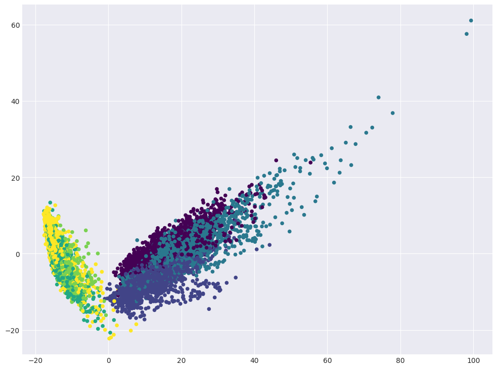
Question 3:
If everything worked out correctly, you will see a number of clusters, almost perfectly separated from each other. What types of activity are included in these clusters?
Answer options:
1 cluster: all 6 activities
2 clusters: (walking, walking upstairs, walking downstairs) and (sitting, standing, laying) [+]
3 clusters: (walking), (walking upstairs, walking downstairs) and (sitting, standing, laying)
6 clusters
Perform clustering with the KMeans method, training the model on data with reduced dimensionality (by PCA). In this case, we will give a clue to look for exactly 6 clusters, but in the general case we will not know how many clusters we should be looking for.
Options:
n_clusters= n_classes (number of unique labels of the target class)n_init= 100random_state= RANDOM_STATE (for reproducibility of the result)
Other parameters should have default values.
# Your code here
kmeans = KMeans(n_clusters=n_classes, n_init=100, random_state=RANDOM_STATE)
kmeans.fit(X_pca)
cluster_labels = kmeans.labels_
Visualize data in projection on the first two principal components. Color the dots according to the clusters obtained.
# Your code here
plt.scatter(X_pca[:, 0], X_pca[:, 1], c=cluster_labels, s=20, cmap="viridis");
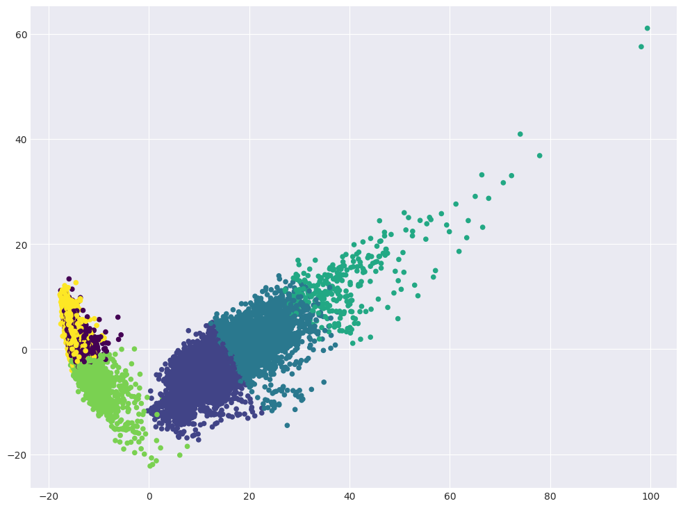
Look at the correspondence between the cluster marks and the original class labels and what kinds of activities the KMeans algorithm is confused at.
tab = pd.crosstab(y, cluster_labels, margins=True)
tab.index = [
    "walking",
    "going up the stairs",
    "going down the stairs",
    "sitting",
    "standing",
    "laying",
    "all",
]
tab.columns = ["cluster" + str(i + 1) for i in range(6)] + ["all"]
tab
| cluster1 | cluster2 | cluster3 | cluster4 | cluster5 | cluster6 | all | |
|---|---|---|---|---|---|---|---|
| walking | 0 | 903 | 741 | 78 | 0 | 0 | 1722 |
| going up the stairs | 0 | 1241 | 296 | 5 | 2 | 0 | 1544 |
| going down the stairs | 0 | 320 | 890 | 196 | 0 | 0 | 1406 |
| sitting | 1235 | 1 | 0 | 0 | 450 | 91 | 1777 |
| standing | 1344 | 0 | 0 | 0 | 562 | 0 | 1906 |
| laying | 52 | 5 | 0 | 0 | 329 | 1558 | 1944 |
| all | 2631 | 2470 | 1927 | 279 | 1343 | 1649 | 10299 |
We see that for each class (i.e., each activity) there are several clusters. Let’s look at the maximum percentage of objects in a class that are assigned to a single cluster. This will be a simple metric that characterizes how easily the class is separated from others when clustering.
Example: if for class “walking downstairs” (with 1406 instances belonging to it), the distribution of clusters is:
cluster 1 - 900
cluster 3 - 500
cluster 6 - 6,
then such a share will be 900/1406 \( \approx \) 0.64.
Question 4:
Which activity is separated from the rest better than others based on the simple metric described above?
Answer options:
walking
standing
walking downstairs
all three options are incorrect [+]
pd.Series(
    tab.iloc[:-1, :-1].max(axis=1).values / tab.iloc[:-1, -1].values,
    index=tab.index[:-1],
)
walking                  0.524390
going up the stairs      0.803756
going down the stairs    0.633001
sitting                  0.694992
standing                 0.705142
laying                   0.801440
dtype: float64
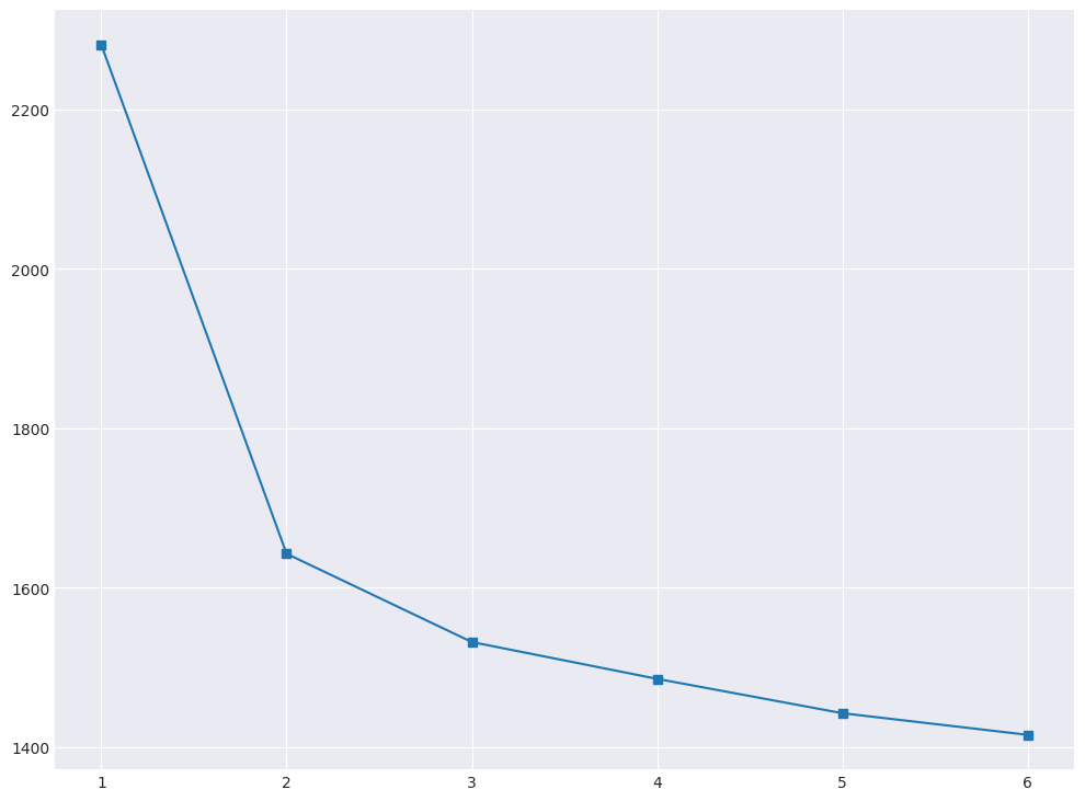
It can be seen that kMeans does not distinguish activities very well. Use the elbow method to select the optimal number of clusters. Parameters of the algorithm and the data we use are the same as before, we change only n_clusters.
# Your code here
inertia = []
for k in tqdm(range(1, n_classes + 1)):
    kmeans = KMeans(n_clusters=k, n_init=100, random_state=RANDOM_STATE).fit(
        X_pca
    )
    inertia.append(np.sqrt(kmeans.inertia_))
plt.plot(range(1, 7), inertia, marker="s");
We calculate \( D(k) \), as described in this article in the section “Choosing the number of clusters for K-means”.
d = {}
for k in range(2, 6):
    i = k - 1
    d[k] = (inertia[i] - inertia[i + 1]) / (inertia[i - 1] - inertia[i])
d
{2: np.float64(0.17344753560094128),
 3: np.float64(0.41688555755864304),
 4: np.float64(0.9332198909748705),
 5: np.float64(0.6297014287707848)}
Question 5:
How many clusters can we choose according to the elbow method?
Answer options:
1
2 [+]
3
4
Let’s try another clustering algorithm, described in the article – agglomerative clustering.
ag = AgglomerativeClustering(n_clusters=n_classes, linkage="ward").fit(X_pca)
Calculate the Adjusted Rand Index (sklearn.metrics) for the resulting clustering and for KMeans with the parameters from the 4th question.
# Your code here
print("KMeans: ARI =", metrics.adjusted_rand_score(y, cluster_labels))
print("Agglomerative CLustering: ARI =", metrics.adjusted_rand_score(y, ag.labels_))
KMeans: ARI = 0.4198070012602345
Agglomerative CLustering: ARI = 0.49362763373004886
Question 6:
Select all the correct statements.
Answer options:
According to ARI, KMeans handled clustering worse than Agglomerative Clustering [+]
For ARI, it does not matter which tags are assigned to the cluster, only the partitioning of instances into clusters matters [+]
In case of random partitioning into clusters, ARI will be close to zero [+]
Comment:
Yes, the higher ARI, the better
Yes, if you renumber clusters differently, ARI will not change
True
You can notice that the task is not very well solved when we try to detect several clusters (> 2). Now, let’s solve the classification problem, given that the data is labeled.
For classification, use the support vector machine – class sklearn.svm.LinearSVC. In this course, we didn’t study this algorithm separately, but it is well-known and you can read about it, for example here.
Choose the C hyperparameter for LinearSVC using GridSearchCV.
Train the new
StandardScaleron the training set (with all original features), apply scaling to the test setIn
GridSearchCV, specifycv= 3.
# Your code here
scaler = StandardScaler()
X_train_scaled = scaler.fit_transform(X_train)
X_test_scaled = scaler.transform(X_test)
svc = LinearSVC(random_state=RANDOM_STATE)
svc_params = {"C": [0.001, 0.01, 0.1, 1, 10]}
%%time
# Your code here
best_svc = GridSearchCV(svc, svc_params, n_jobs=4, cv=3, verbose=1)
best_svc.fit(X_train_scaled, y_train);
Fitting 3 folds for each of 5 candidates, totalling 15 fits
/Users/kashnitsky/Documents/misc/mlcourse.ai/.venv/lib/python3.13/site-packages/sklearn/svm/_base.py:1249: ConvergenceWarning: Liblinear failed to converge, increase the number of iterations.
  warnings.warn(
/Users/kashnitsky/Documents/misc/mlcourse.ai/.venv/lib/python3.13/site-packages/sklearn/svm/_base.py:1249: ConvergenceWarning: Liblinear failed to converge, increase the number of iterations.
  warnings.warn(
/Users/kashnitsky/Documents/misc/mlcourse.ai/.venv/lib/python3.13/site-packages/sklearn/svm/_base.py:1249: ConvergenceWarning: Liblinear failed to converge, increase the number of iterations.
  warnings.warn(
CPU times: user 2.17 s, sys: 62.3 ms, total: 2.23 s
Wall time: 21.9 s
best_svc.best_params_, best_svc.best_score_
({'C': 0.1}, np.float64(0.9379785010699506))
Question 7
Which value of the hyperparameter C was chosen the best on the basis of cross-validation?
Answer options:
0.001
0.01
0.1 [+]
1
10
y_predicted = best_svc.predict(X_test_scaled)
tab = pd.crosstab(y_test, y_predicted, margins=True)
tab.index = [
    "walking",
    "climbing up the stairs",
    "going down the stairs",
    "sitting",
    "standing",
    "laying",
    "all",
]
tab.columns = [
    "walking",
    "climbing up the stairs",
    "going down the stairs",
    "sitting",
    "standing",
    "laying",
    "all",
]
tab
| walking | climbing up the stairs | going down the stairs | sitting | standing | laying | all | |
|---|---|---|---|---|---|---|---|
| walking | 494 | 2 | 0 | 0 | 0 | 0 | 496 |
| climbing up the stairs | 12 | 459 | 0 | 0 | 0 | 0 | 471 |
| going down the stairs | 2 | 4 | 413 | 1 | 0 | 0 | 420 |
| sitting | 0 | 4 | 0 | 426 | 61 | 0 | 491 |
| standing | 0 | 0 | 0 | 15 | 517 | 0 | 532 |
| laying | 0 | 0 | 0 | 0 | 11 | 526 | 537 |
| all | 508 | 469 | 413 | 442 | 589 | 526 | 2947 |
As you can see, the classification problem is solved quite well.
Question 8:
Which activity type is worst detected by SVM in terms of precision? Recall?
Answer options:
precision – going up the stairs, recall – laying
precision – laying, recall – sitting
precision – walking, recall – walking
precision – standing, recall – sitting [+]
Comment: The classifier solved the problem well, but not ideally.
Finally, do the same thing as in Question 7, but add PCA.
Use
X_train_scaledandX_test_scaledTrain the same PCA as before, on the scaled training set, apply scaling to the test set
Choose the hyperparameter
Cvia cross-validation on the training set with PCA-transformation. You will notice how much faster it works now.
Question 9:
What is the difference between the best quality (accuracy) for cross-validation in the case of all 561 initial characteristics and in the second case, when the principal component method was applied? Round to the nearest percent.
Answer options:
quality is the same
2%
4% [+]
10%
20%
# Your code here
scaler = StandardScaler()
X_train_scaled = scaler.fit_transform(X_train)
X_test_scaled = scaler.transform(X_test)

pca = PCA(n_components=0.9, random_state=RANDOM_STATE)
X_train_pca = pca.fit_transform(X_train_scaled)
X_test_pca = pca.transform(X_test_scaled)
svc = LinearSVC(random_state=RANDOM_STATE, max_iter=5000)
svc_params = {"C": [0.001, 0.01, 0.1, 1, 10]}
%%time
best_svc_pca = GridSearchCV(svc, svc_params, n_jobs=4, cv=3, verbose=1)
best_svc_pca.fit(X_train_pca, y_train);
Fitting 3 folds for each of 5 candidates, totalling 15 fits
CPU times: user 140 ms, sys: 4.88 ms, total: 145 ms
Wall time: 825 ms
best_svc_pca.best_params_, best_svc_pca.best_score_
({'C': 0.1}, np.float64(0.8983982658750974))
The result with PCA is worse by 4%, comparing accuracy on cross-validation.
round(100 * (best_svc_pca.best_score_ - best_svc.best_score_))
-4
Question 10:
Select all the correct statements:
Answer options:
Principal component analysis in this case allowed us to reduce the model training time, while the quality (mean cross-validation accuracy) suffered greatly, by more than 10%
PCA can be used to visualize data, but there are better methods for this task, for example, tSNE. However, PCA has lower computational complexity [+]
PCA builds linear combinations of initial features, and in some applications they might be poorly interpreted by humans [+]
Comment:
The first statement is true, principal component analysis in this case allowed us to significantly reduce the training time of the model, but the quality suffered not so much – by only 4%
For multidimensional data visualization it is better to use manifold learning methods, in particular, tSNE. At the same time, metrics assessing the quality of visualization have not really been invented yet, but tSNE is widely used precisely because in some cases it builds “good” pictures showing the data structure, as in the case of MNIST
Linear combinations of features, that PCA builds, are often poorly interpreted by humans, for example, 0.574 * salary + 0.234 * num_children